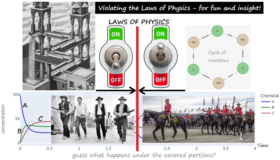
Violating the Laws of Physics for Fun and Insight!¶

A cascade of reactions `A <-> B <-> C` , mostly in the forward direction¶

PART 1 : the above, together with a PHYSICALLY-IMPOSSIBLE "closing" of the cycle with :¶

`C <-> A`, ALSO mostly in the forward direction (never mind the laws of thermodymics)!¶

PART 2 : restoring the law of physics (by letting `C <-> A` adjust its kinetics based on the energy difference.)¶

All 1st-order kinetics.

LAST REVISED: June 23, 2024 (using v. 1.0 beta36)

Temporarily suspending the Laws of Physics

In [1]:

import set_path      # Importing this module will add the project's home directory to sys.path

Added 'D:\Docs\- MY CODE\BioSimulations\life123-Win7' to sys.path

In [2]:

from experiments.get_notebook_info import get_notebook_basename

from life123 import ChemData as chem
from life123 import UniformCompartment

import plotly.express as px
import plotly.graph_objects as go
from life123 import GraphicLog

In [3]:

# Initialize the HTML logging
log_file = get_notebook_basename() + ".log.htm"    # Use the notebook base filename for the log file

# Set up the use of some specified graphic (Vue) components
GraphicLog.config(filename=log_file,
                  components=["vue_cytoscape_2"],
                  extra_js="https://cdnjs.cloudflare.com/ajax/libs/cytoscape/3.21.2/cytoscape.umd.js")

-> Output will be LOGGED into the file 'impossible_1.log.htm'

Initialize the system¶

In [4]:

# Initialize the system
chem_data = chem(names=["A", "B", "C"])

# Reaction A <-> B, mostly in forward direction (favored energetically)
# Note: all reactions in this experiment have 1st-order kinetics for all species
chem_data.add_reaction(reactants="A", products="B",
                       forward_rate=9., reverse_rate=3.)

# Reaction B <-> C, also favored energetically
chem_data.add_reaction(reactants="B", products="C",
                       forward_rate=8., reverse_rate=4.)

Out[4]:

Part 1 - "Turning off the Laws of Physics"!¶

In [5]:

# LET'S VIOLATE THE LAWS OF PHYSICS!
# Reaction C <-> A, also mostly in forward direction - MAGICALLY GOING "UPSTREAM" from C, to the higher-energy level of "A"
chem_data.add_reaction(reactants="C" , products="A",
                       forward_rate=3., reverse_rate=2.) # *** PHYSICALLY IMPOSSIBLE! *** Future versions of Life123 may flag this!

chem_data.describe_reactions()

# Send the plot of the reaction network to the HTML log file
chem_data.plot_reaction_network("vue_cytoscape_2")

Number of reactions: 3 (at temp. 25 C)
0: A <-> B  (kF = 9 / kR = 3 / delta_G = -2,723.4 / K = 3) | 1st order in all reactants & products
1: B <-> C  (kF = 8 / kR = 4 / delta_G = -1,718.3 / K = 2) | 1st order in all reactants & products
2: C <-> A  (kF = 3 / kR = 2 / delta_G = -1,005.1 / K = 1.5) | 1st order in all reactants & products
Set of chemicals involved in the above reactions: {'A', 'B', 'C'}
[GRAPHIC ELEMENT SENT TO LOG FILE `impossible_1.log.htm`]

Notice the absurdity of the energy levels always going down, throughout the cycle (like in an Escher painting!)¶

Energy levels always going down

Set the initial concentrations of all the chemicals¶

In [6]:

initial_conc = {"A": 100.} 
initial_conc

Out[6]:

{'A': 100.0}

In [7]:

dynamics = UniformCompartment(chem_data=chem_data)
dynamics.set_conc(conc=initial_conc, snapshot=True)
dynamics.describe_state()

SYSTEM STATE at Time t = 0:
3 species:
  Species 0 (A). Conc: 100.0
  Species 1 (B). Conc: 0.0
  Species 2 (C). Conc: 0.0
Set of chemicals involved in reactions: {'A', 'B', 'C'}

In [8]:

dynamics.set_diagnostics()       # To save diagnostic information about the call to single_compartment_react()

dynamics.single_compartment_react(initial_step=0.01, target_end_time=2.0,
                                  variable_steps=False)   # To avoid extra complexity, we're sticking to simple fixed-time steps

200 total step(s) taken

In [9]:

dynamics.plot_history()

In [10]:

# dynamics.explain_time_advance()

# dynamics.get_history()

It might look like an equilibrium has been reached. But NOT! Verify the LACK of final equilibrium state:¶

In [11]:

dynamics.is_in_equilibrium()

0: A <-> B
Final concentrations: [A] = 21.43 ; [B] = 33.81
1. Ratio of reactant/product concentrations, adjusted for reaction orders: 1.57778
    Formula used:  [B] / [A]
2. Ratio of forward/reverse reaction rates: 3
Discrepancy between the two values: 47.41 %
Reaction is NOT in equilibrium (not within 1% tolerance)

1: B <-> C
Final concentrations: [B] = 33.81 ; [C] = 44.76
1. Ratio of reactant/product concentrations, adjusted for reaction orders: 1.32394
    Formula used:  [C] / [B]
2. Ratio of forward/reverse reaction rates: 2
Discrepancy between the two values: 33.8 %
Reaction is NOT in equilibrium (not within 1% tolerance)

2: C <-> A
Final concentrations: [C] = 44.76 ; [A] = 21.43
1. Ratio of reactant/product concentrations, adjusted for reaction orders: 0.478723
    Formula used:  [A] / [C]
2. Ratio of forward/reverse reaction rates: 1.5
Discrepancy between the two values: 68.09 %
Reaction is NOT in equilibrium (not within 1% tolerance)

Out[11]:

{False: [0, 1, 2]}

Not surprisingly, none of the reactions of this physically-impossible hypothetical system are in equilibrium¶

Even though the concentrations don't change, it's NOT from equilibrium in the reactions - but rather from a balancing out of consuming and replenishing across reactions.¶

Consider, for example, the concentrations of the chemical `A` at the end time, and contributions to its change ("Delta A") from the individual reactions affecting `A`, as available from the diagnostic data:¶

In [12]:

dynamics.get_diagnostic_rxn_data(rxn_index=0, tail=3)

Reaction:  A <-> B

Out[12]:

	START_TIME	Delta A	Delta B	time_step
197	1.97	-0.914286	0.914286	0.01
198	1.98	-0.914286	0.914286	0.01
199	1.99	-0.914286	0.914286	0.01

In [13]:

dynamics.get_diagnostic_rxn_data(rxn_index=2, tail=3)

Reaction:  C <-> A

Out[13]:

	START_TIME	Delta A	Delta C	time_step
197	1.97	0.914286	-0.914286	0.01
198	1.98	0.914286	-0.914286	0.01
199	1.99	0.914286	-0.914286	0.01

Looking at the last row from each of the 2 dataframes above, one case see that, at every reaction cycle, [A] gets reduced by some quantity (0.914286) by the reaction `A <-> B`, while simultaneously getting increased by the SAME amount by the (fictional) reaction `C <-> A`.¶

Hence, the concentration of A remains constant - but none of the reactions is in equilibrium!¶

In [ ]:

PART 2 - Let's restore the Laws of Physics!¶

In [14]:

chem_data.describe_reactions()

Number of reactions: 3 (at temp. 25 C)
0: A <-> B  (kF = 9 / kR = 3 / delta_G = -2,723.4 / K = 3) | 1st order in all reactants & products
1: B <-> C  (kF = 8 / kR = 4 / delta_G = -1,718.3 / K = 2) | 1st order in all reactants & products
2: C <-> A  (kF = 3 / kR = 2 / delta_G = -1,005.1 / K = 1.5) | 1st order in all reactants & products
Set of chemicals involved in the above reactions: {'A', 'B', 'C'}

In [15]:

dynamics.clear_reactions()       # Let's start over with the reactions  (without affecting the data from the reactions)

In [16]:

# For the reactions A <-> B, and B <-> C, everything is being restored to the way it was before
chem_data.add_reaction(reactants="A", products="B",
                       forward_rate=9., reverse_rate=3.)

# Reaction , also favored energetically
chem_data.add_reaction(reactants="B", products="C",
                       forward_rate=8., reverse_rate=4.)

Out[16]:

In [17]:

chem_data.describe_reactions()

Number of reactions: 2 (at temp. 25 C)
0: A <-> B  (kF = 9 / kR = 3 / delta_G = -2,723.4 / K = 3) | 1st order in all reactants & products
1: B <-> C  (kF = 8 / kR = 4 / delta_G = -1,718.3 / K = 2) | 1st order in all reactants & products
Set of chemicals involved in the above reactions: {'A', 'C', 'B'}

In [18]:

# But for the reaction C <-> A, this time we'll "bend the knee" to the laws of thermodynamics!
# We'll use the same forward rate as before, but we'll let the reverse rate be picked by the system, 
# based of thermodynamic data consistent with the previous 2 reactions : i.e. an energy difference of -(-2,723.41 - 1,718.28) = +4,441.69 (reflecting the  
# "going uphill energetically" from C to A
chem_data.add_reaction(reactants="C", products="A",
                       forward_rate=3., delta_G=4441.69)   # Notice the positive Delta G: we're going from "C", to the higher-energy level of "A"

Out[18]:

In [19]:

chem_data.describe_reactions()

Number of reactions: 3 (at temp. 25 C)
0: A <-> B  (kF = 9 / kR = 3 / delta_G = -2,723.4 / K = 3) | 1st order in all reactants & products
1: B <-> C  (kF = 8 / kR = 4 / delta_G = -1,718.3 / K = 2) | 1st order in all reactants & products
2: C <-> A  (kF = 3 / kR = 18 / delta_G = 4,441.7 / K = 0.16667) | 1st order in all reactants & products
Set of chemicals involved in the above reactions: {'A', 'B', 'C'}

Notice how, now that we're again following the laws of thermodynamics, the last reaction is mostly IN REVERSE (low K < 1), as it ought to be!¶

(considering how energetically unfavorable it is)¶

Now, let's continue with this "legit" set of reactions, from where we left off in our fantasy world at time t=2:¶

In [20]:

dynamics.single_compartment_react(initial_step=0.005, target_end_time=4.0,
                                  variable_steps=False)

#dynamics.explain_time_advance()

#dynamics.get_history()

400 total step(s) taken

In [21]:

fig0 = dynamics.plot_history()   # Prepare, but don't show, the main plot

In [22]:

# Add a second plot, with a vertical gray line at t=2
fig1 = px.line(x=[2,2], y=[0,100], color_discrete_sequence = ['gray'])

# Combine the plots, and display them
all_fig = go.Figure(data=fig0.data + fig1.data, layout = fig0.layout)    # Note that the + is concatenating lists
all_fig.update_layout(title="On the left of vertical gray line: FICTIONAL world; on the right: REAL world!")
all_fig.show()

Notice how [A] drops at time t=2, when we re-enact the Laws of Physics, because A no longer receives the extra boost from the previous mostly-forward (and thus physically-impossible given the unfavorable energy levels!) reaction `C <-> A`.¶

Back to the real world, that (energetically unfavored) reaction now mostly goes IN REVERSE; hence, the boost in [C] as well¶

Now, we have a REAL equilibrium!¶

In [23]:

dynamics.is_in_equilibrium()

0: A <-> B
Final concentrations: [A] = 10 ; [B] = 30
1. Ratio of reactant/product concentrations, adjusted for reaction orders: 3
    Formula used:  [B] / [A]
2. Ratio of forward/reverse reaction rates: 3
Discrepancy between the two values: 0.0001018 %
Reaction IS in equilibrium (within 1% tolerance)

1: B <-> C
Final concentrations: [B] = 30 ; [C] = 60
1. Ratio of reactant/product concentrations, adjusted for reaction orders: 2
    Formula used:  [C] / [B]
2. Ratio of forward/reverse reaction rates: 2
Discrepancy between the two values: 3.817e-05 %
Reaction IS in equilibrium (within 1% tolerance)

2: C <-> A
Final concentrations: [C] = 60 ; [A] = 10
1. Ratio of reactant/product concentrations, adjusted for reaction orders: 0.166667
    Formula used:  [A] / [C]
2. Ratio of forward/reverse reaction rates: 0.166667
Discrepancy between the two values: 5.09e-05 %
Reaction IS in equilibrium (within 1% tolerance)

Out[23]:

True

The fact that individual reactions are now in actual, real equilibrium, can be easily seen from the last rows in the diagnostic data. Notice all the delta-concentration values at the final times are virtually zero:¶

In [24]:

dynamics.get_diagnostic_rxn_data(rxn_index=0, tail=1)

Reaction:  A <-> B

Out[24]:

	START_TIME	Delta A	Delta B	Delta C	time_step	caption
599	3.995	-4.580895e-07	4.580895e-07	0.0	0.005

In [25]:

dynamics.get_diagnostic_rxn_data(rxn_index=1, tail=1)

Reaction:  B <-> C

Out[25]:

	START_TIME	Delta A	Delta B	Delta C	time_step	caption
599	3.995	0.0	-4.580895e-07	4.580895e-07	0.005

In [26]:

dynamics.get_diagnostic_rxn_data(rxn_index=2, tail=1)

Reaction:  C <-> A

Out[26]:

	START_TIME	Delta A	Delta B	Delta C	time_step	caption
599	3.995	4.580895e-07	0.0	-4.580895e-07	0.005