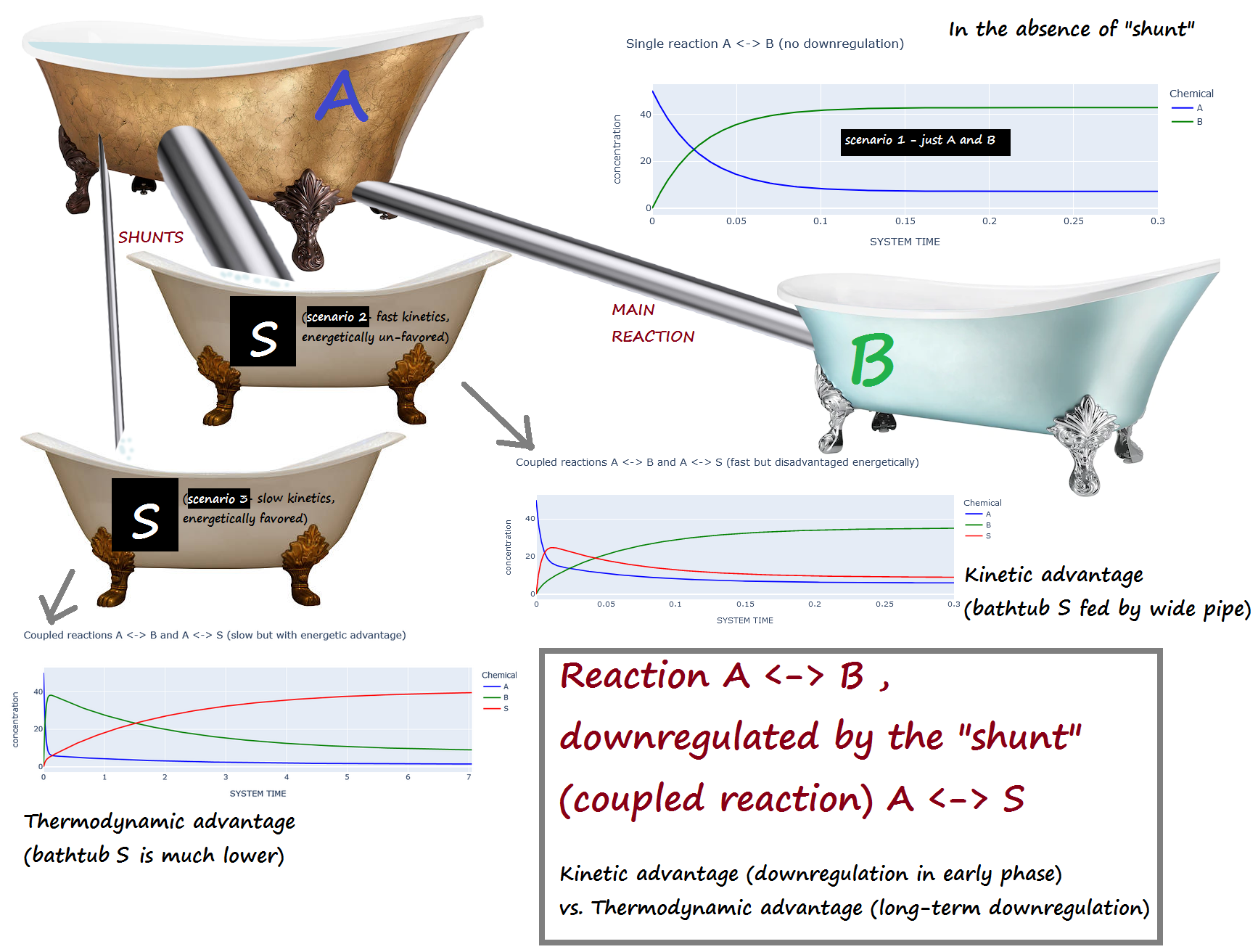
`A <-> B` , downregulated by the "shunt" (coupled reaction) `A <-> S`¶

Kinetic advantage (downregulation in early phase) vs. Thermodynamic advantage (long-term downregulation)¶

Scenario 1 : No downregulation on A <-> B

Scenario 2 : The shunt (A <-> S) has a kinetic advantage but thermodynamic DIS-advantage compared to A <-> B
(i.e. A <-> S is fast, but energetically unfavored)

Scenario 3 : The shunt (A <-> S) is has a kinetic DIS-advantage but a thermodynamic advantage compared to A <-> B
(i.e. A <-> S is slow, but energetically favored)

All reactions are 1st order, mostly forward. Taken to equilibrium.

LAST REVISED: June 23, 2024 (using v. 1.0 beta36)

Bathtub analogy:¶

A is initially full, while B and S are empty.
If the "shunt" S is present, scenario 2 corresponds to a large pipe and a small elevation change...
while scenario 3 corresponds to a narrow pipe and a large elevation change.

Downregulated by shunt

In [1]:

import set_path      # Importing this module will add the project's home directory to sys.path

Added 'D:\Docs\- MY CODE\BioSimulations\life123-Win7' to sys.path

In [2]:

from experiments.get_notebook_info import get_notebook_basename

from life123 import ChemData as chem
from life123 import UniformCompartment

import plotly.express as px
from life123 import GraphicLog

In [3]:

# Initialize the HTML logging (for the graphics)
log_file = get_notebook_basename() + ".log.htm"    # Use the notebook base filename for the log file

# Set up the use of some specified graphic (Vue) components
GraphicLog.config(filename=log_file,
                  components=["vue_cytoscape_2"],
                  extra_js="https://cdnjs.cloudflare.com/ajax/libs/cytoscape/3.21.2/cytoscape.umd.js")

-> Output will be LOGGED into the file 'down_regulate_1.log.htm'

In [ ]:

Scenario 1: A <-> B in the absence of the 2nd reaction ¶

Initialize the System¶

Specify the chemicals and the reaction

In [4]:

# Specify the chemicals
chem_data = chem(names=["A", "B"])

# Reaction A <-> B
chem_data.add_reaction(reactants=["A"], products=["B"],
                       forward_rate=30., reverse_rate=5.)

chem_data.describe_reactions()

Number of reactions: 1 (at temp. 25 C)
0: A <-> B  (kF = 30 / kR = 5 / delta_G = -4,441.7 / K = 6) | 1st order in all reactants & products
Set of chemicals involved in the above reactions: {'A', 'B'}

Set the initial concentrations of all the chemicals¶

In [5]:

dynamics = UniformCompartment(chem_data=chem_data, preset="fast")
dynamics.set_conc(conc={"A": 50.}, snapshot=True)
dynamics.describe_state()

SYSTEM STATE at Time t = 0:
2 species:
  Species 0 (A). Conc: 50.0
  Species 1 (B). Conc: 0.0
Set of chemicals involved in reactions: {'A', 'B'}

Run the reaction¶

In [6]:

dynamics.set_diagnostics()          # To save diagnostic information about the call to single_compartment_react()

# The changes of concentrations vary very rapidly early on; automated variable timesteps will take care of that
dynamics.single_compartment_react(initial_step=0.001, duration=0.3,
                                  snapshots={"initial_caption": "1st reaction step",
                                             "final_caption": "last reaction step"},
                                  variable_steps=True)

37 total step(s) taken
Number of step re-do's because of negative concentrations: 0
Number of step re-do's because of elective soft aborts: 0
Norm usage: {'norm_A': 22, 'norm_B': 17, 'norm_C': 16, 'norm_D': 16}

In [7]:

dynamics.get_history()

Out[7]:

	SYSTEM TIME	A	B	caption
0	0.000000	50.000000	0.000000	Initialized state
1	0.001000	48.500000	1.500000	1st reaction step
2	0.002000	47.052500	2.947500
3	0.002800	45.935030	4.064970
4	0.003600	44.848849	5.151151
5	0.004400	43.793081	6.206919
6	0.005200	42.766875	7.233125
7	0.006000	41.769403	8.230597
8	0.007200	40.315088	9.684912
9	0.008400	38.921854	11.078146
10	0.009600	37.587136	12.412864
11	0.010800	36.308476	13.691524
12	0.012000	35.083520	14.916480
13	0.013800	33.323259	16.676741
14	0.015240	32.003766	17.996234
15	0.016680	30.750777	19.249223
16	0.018840	28.966018	21.033982
17	0.020568	27.646153	22.353847
18	0.022296	26.406114	23.593886
19	0.024888	24.658551	25.341449
20	0.026962	23.387332	26.612668
21	0.029035	22.208373	27.791627
22	0.032146	20.568281	29.431719
23	0.034634	19.399045	30.600955
24	0.038366	17.797935	32.202065
25	0.041352	16.684379	33.315621
26	0.045831	15.188610	34.811390
27	0.050310	13.927325	36.072675
28	0.057029	12.331983	37.668017
29	0.062404	11.355820	38.644180
30	0.070466	10.167025	39.832975
31	0.082559	8.887006	41.112994
32	0.094652	8.148772	41.851228
33	0.112792	7.510122	42.489878
34	0.140002	7.160360	42.839640
35	0.180816	7.135357	42.864643
36	0.242039	7.151428	42.848572
37	0.333872	7.123879	42.876121	last reaction step

In [8]:

dynamics.explain_time_advance()

From time 0 to 0.002, in 2 steps of 0.001
From time 0.002 to 0.006, in 5 steps of 0.0008
From time 0.006 to 0.012, in 5 steps of 0.0012
From time 0.012 to 0.0138, in 1 step of 0.0018
From time 0.0138 to 0.01668, in 2 steps of 0.00144
From time 0.01668 to 0.01884, in 1 step of 0.00216
From time 0.01884 to 0.0223, in 2 steps of 0.00173
From time 0.0223 to 0.02489, in 1 step of 0.00259
From time 0.02489 to 0.02904, in 2 steps of 0.00207
From time 0.02904 to 0.03215, in 1 step of 0.00311
From time 0.03215 to 0.03463, in 1 step of 0.00249
From time 0.03463 to 0.03837, in 1 step of 0.00373
From time 0.03837 to 0.04135, in 1 step of 0.00299
From time 0.04135 to 0.05031, in 2 steps of 0.00448
From time 0.05031 to 0.05703, in 1 step of 0.00672
From time 0.05703 to 0.0624, in 1 step of 0.00537
From time 0.0624 to 0.07047, in 1 step of 0.00806
From time 0.07047 to 0.09465, in 2 steps of 0.0121
From time 0.09465 to 0.1128, in 1 step of 0.0181
From time 0.1128 to 0.14, in 1 step of 0.0272
From time 0.14 to 0.1808, in 1 step of 0.0408
From time 0.1808 to 0.242, in 1 step of 0.0612
From time 0.242 to 0.3339, in 1 step of 0.0918
(37 steps total)

In [9]:

dynamics.plot_history(colors=["darkturquoise", "green"], title="Single reaction A <-> B (no downregulation)",
                      show_intervals=True)

Notice the intersection at the exact midpoint of the 2 initial concentrations (50 and 0):¶

In [10]:

dynamics.curve_intersect('A', 'B', t_start=0, t_end=0.1)

Out[10]:

(0.024381560069949713, 25.0)

In [11]:

# Verify that all the reactions have reached equilibrium
dynamics.is_in_equilibrium()

0: A <-> B
Final concentrations: [A] = 7.124 ; [B] = 42.88
1. Ratio of reactant/product concentrations, adjusted for reaction orders: 6.01865
    Formula used:  [B] / [A]
2. Ratio of forward/reverse reaction rates: 6
Discrepancy between the two values: 0.3108 %
Reaction IS in equilibrium (within 1% tolerance)

Out[11]:

True

In [ ]:

Scenario 2 - downregulated by shunt:¶

kinetically fast,¶

but with thermodynamical dis-advantage (i.e. energetically un-favored)¶

In [12]:

# Register the new chemical ("S")
chem_data.add_chemical("S")

# Add the reaction A <-> S (fast shunt, poor thermodynical energetic advantage)
chem_data.add_reaction(reactants=["A"], products=["S"],
                       forward_rate=150., reverse_rate=100.) 

chem_data.describe_reactions()

Number of reactions: 2 (at temp. 25 C)
0: A <-> B  (kF = 30 / kR = 5 / delta_G = -4,441.7 / K = 6) | 1st order in all reactants & products
1: A <-> S  (kF = 150 / kR = 100 / delta_G = -1,005.1 / K = 1.5) | 1st order in all reactants & products
Set of chemicals involved in the above reactions: {'S', 'A', 'B'}

In [13]:

# Send a plot of the network of reactions to the HTML log file
chem_data.plot_reaction_network("vue_cytoscape_2")

[GRAPHIC ELEMENT SENT TO LOG FILE `down_regulate_1.log.htm`]

In [14]:

dynamics = UniformCompartment(chem_data=chem_data, preset="mid")   # Notice we're over-writing the earlier "dynamics" object
dynamics.set_conc(conc={"A": 50.}, snapshot=True)
dynamics.describe_state()

SYSTEM STATE at Time t = 0:
3 species:
  Species 0 (A). Conc: 50.0
  Species 1 (B). Conc: 0.0
  Species 2 (S). Conc: 0.0
Set of chemicals involved in reactions: {'S', 'A', 'B'}

Run the reaction¶

In [15]:

dynamics.set_diagnostics()         # To save diagnostic information about the call to single_compartment_react()

# The changes of concentrations vary very rapidly early on; automated variable timesteps will take care of that
dynamics.single_compartment_react(initial_step=0.001, duration=0.3,
                                  snapshots={"initial_caption": "1st reaction step",
                                             "final_caption": "last reaction step"},
                                  variable_steps=True)

57 total step(s) taken
Number of step re-do's because of negative concentrations: 0
Number of step re-do's because of elective soft aborts: 2
Norm usage: {'norm_A': 38, 'norm_B': 37, 'norm_C': 36, 'norm_D': 36}

In [16]:

dynamics.plot_history(colors=["darkturquoise", "green", "red"],
                      title="Coupled reactions A <-> B and A <-> S (fast but disadvantaged energetically)",
                      show_intervals=True)

Notice how the "alternate (shunt) path" of the reaction, i.e. S (red)¶

has a FAST START (fast kinetics),¶

but EVENTUALLY PETERS OUT (energy dis-advantage)¶

In [17]:

# Verify that all the reactions have reached equilibrium
dynamics.is_in_equilibrium()

0: A <-> B
Final concentrations: [A] = 5.887 ; [B] = 35.24
1. Ratio of reactant/product concentrations, adjusted for reaction orders: 5.98644
    Formula used:  [B] / [A]
2. Ratio of forward/reverse reaction rates: 6
Discrepancy between the two values: 0.226 %
Reaction IS in equilibrium (within 1% tolerance)

1: A <-> S
Final concentrations: [A] = 5.887 ; [S] = 8.873
1. Ratio of reactant/product concentrations, adjusted for reaction orders: 1.50724
    Formula used:  [S] / [A]
2. Ratio of forward/reverse reaction rates: 1.5
Discrepancy between the two values: 0.4824 %
Reaction IS in equilibrium (within 1% tolerance)

Out[17]:

True

In [ ]:

Scenario 3 - downregulated by shunt:¶

kinetically slow,¶

but with thermodynamical advantage (i.e. energetically favored)¶

In [18]:

# Specify the chemicals  (notice that we're starting with new objects)
new_chem_data = chem(names=["A", "B", "S"])

# Reaction A <-> B (as before)
new_chem_data.add_reaction(reactants=["A"], products=["B"],
                       forward_rate=30., reverse_rate=5.) 

# Reaction A <-> S (slow shunt, excellent thermodynamical energetic advantage)
new_chem_data.add_reaction(reactants=["A"], products=["S"],
                       forward_rate=3., reverse_rate=0.1)

new_chem_data.describe_reactions()

Number of reactions: 2 (at temp. 25 C)
0: A <-> B  (kF = 30 / kR = 5 / delta_G = -4,441.7 / K = 6) | 1st order in all reactants & products
1: A <-> S  (kF = 3 / kR = 0.1 / delta_G = -8,431.4 / K = 30) | 1st order in all reactants & products
Set of chemicals involved in the above reactions: {'S', 'A', 'B'}

In [19]:

dynamics = UniformCompartment(chem_data=new_chem_data, preset="small_rel_change")
dynamics.set_conc(conc={"A": 50.}, snapshot=True)
dynamics.describe_state()

SYSTEM STATE at Time t = 0:
3 species:
  Species 0 (A). Conc: 50.0
  Species 1 (B). Conc: 0.0
  Species 2 (S). Conc: 0.0
Set of chemicals involved in reactions: {'S', 'A', 'B'}

Run the reaction¶

In [20]:

dynamics.set_diagnostics()       # To save diagnostic information about the call to single_compartment_react()

# The changes of concentrations vary very rapidly early on; automated variable timesteps will take care of that
dynamics.single_compartment_react(initial_step=0.005, duration=7.0,
                                  snapshots={"initial_caption": "1st reaction step",
                                             "final_caption": "last reaction step"},
                                  variable_steps=True)

454 total step(s) taken
Number of step re-do's because of negative concentrations: 0
Number of step re-do's because of elective soft aborts: 1
Norm usage: {'norm_A': 17, 'norm_B': 17, 'norm_C': 16, 'norm_D': 16}

In [21]:

dynamics.plot_history(colors=["darkturquoise", "green", "red"],
                      title="Coupled reactions A <-> B and A <-> S (slow but with energetic advantage)")

Notice how the "alternate (shunt) path" of the reaction, i.e. S (red)¶

has a SLOW START (slow kinetics),¶

but EVENTUALLY DOMINATES (energy advantage)¶

In [22]:

dynamics.explain_time_advance()

From time 0 to 0.0025, in 2 steps of 0.00125
From time 0.0025 to 0.03281, in 97 steps of 0.000313
From time 0.03281 to 0.05859, in 55 steps of 0.000469
From time 0.05859 to 0.07617, in 25 steps of 0.000703
From time 0.07617 to 0.09199, in 15 steps of 0.00105
From time 0.09199 to 0.1062, in 9 steps of 0.00158
From time 0.1062 to 0.1205, in 6 steps of 0.00237
From time 0.1205 to 0.2237, in 29 steps of 0.00356
From time 0.2237 to 0.3999, in 33 steps of 0.00534
From time 0.3999 to 0.6402, in 30 steps of 0.00801
From time 0.6402 to 0.9525, in 26 steps of 0.012
From time 0.9525 to 1.349, in 22 steps of 0.018
From time 1.349 to 1.998, in 24 steps of 0.027
From time 1.998 to 3.66, in 41 steps of 0.0405
From time 3.66 to 4.876, in 20 steps of 0.0608
From time 4.876 to 5.971, in 12 steps of 0.0912
From time 5.971 to 6.929, in 7 steps of 0.137
From time 6.929 to 7.134, in 1 step of 0.205
(454 steps total)

Check the final equilibrium¶

In [23]:

# Verify that all the reactions are close to equilibrium
dynamics.is_in_equilibrium(tolerance=12)

0: A <-> B
Final concentrations: [A] = 1.488 ; [B] = 9.019
1. Ratio of reactant/product concentrations, adjusted for reaction orders: 6.06134
    Formula used:  [B] / [A]
2. Ratio of forward/reverse reaction rates: 6
Discrepancy between the two values: 1.022 %
Reaction IS in equilibrium (within 12% tolerance)

1: A <-> S
Final concentrations: [A] = 1.488 ; [S] = 39.49
1. Ratio of reactant/product concentrations, adjusted for reaction orders: 26.5412
    Formula used:  [S] / [A]
2. Ratio of forward/reverse reaction rates: 30
Discrepancy between the two values: 11.53 %
Reaction IS in equilibrium (within 12% tolerance)

Out[23]:

True

Please note the much-longer timescale from the earlier plots¶

If we look at early time interval, this is what it looks like:

In [24]:

dynamics.plot_history(colors=["darkturquoise", "green", "red"],
                      title="Same plot as above, both only showing initial detail", xrange=[0, 0.3])

In [25]:

# Look at where the curves intersect
dynamics.curve_intersect("A", "B", t_start=0, t_end=0.1)

Out[25]:

(0.02405919499545674, 23.73396682504195)

In [26]:

dynamics.curve_intersect("A", "S", t_start=0.1, t_end=0.2)

Out[26]:

(0.14412951669101942, 6.026379520544665)

In [ ]:

A <-> B , downregulated by the "shunt" (coupled reaction) A <-> S¶

Kinetic advantage (downregulation in early phase) vs. Thermodynamic advantage (long-term downregulation)¶

Bathtub analogy:¶

Scenario 1: A <-> B in the absence of the 2nd reaction¶

Initialize the System¶

Set the initial concentrations of all the chemicals¶

Run the reaction¶

Notice the intersection at the exact midpoint of the 2 initial concentrations (50 and 0):¶

Scenario 2 - downregulated by shunt:¶

kinetically fast,¶

but with thermodynamical dis-advantage (i.e. energetically un-favored)¶

Run the reaction¶

Notice how the "alternate (shunt) path" of the reaction, i.e. S (red)¶

has a FAST START (fast kinetics),¶

but EVENTUALLY PETERS OUT (energy dis-advantage)¶

Scenario 3 - downregulated by shunt:¶

kinetically slow,¶

but with thermodynamical advantage (i.e. energetically favored)¶

Run the reaction¶

Notice how the "alternate (shunt) path" of the reaction, i.e. S (red)¶

has a SLOW START (slow kinetics),¶

but EVENTUALLY DOMINATES (energy advantage)¶

Check the final equilibrium¶

Please note the much-longer timescale from the earlier plots¶

`A <-> B` , downregulated by the "shunt" (coupled reaction) `A <-> S`¶

Scenario 1: A <-> B in the absence of the 2nd reaction ¶