Tour of Life123's process of automatic detection - and stepsize reduction - in case any concentration goes negative¶

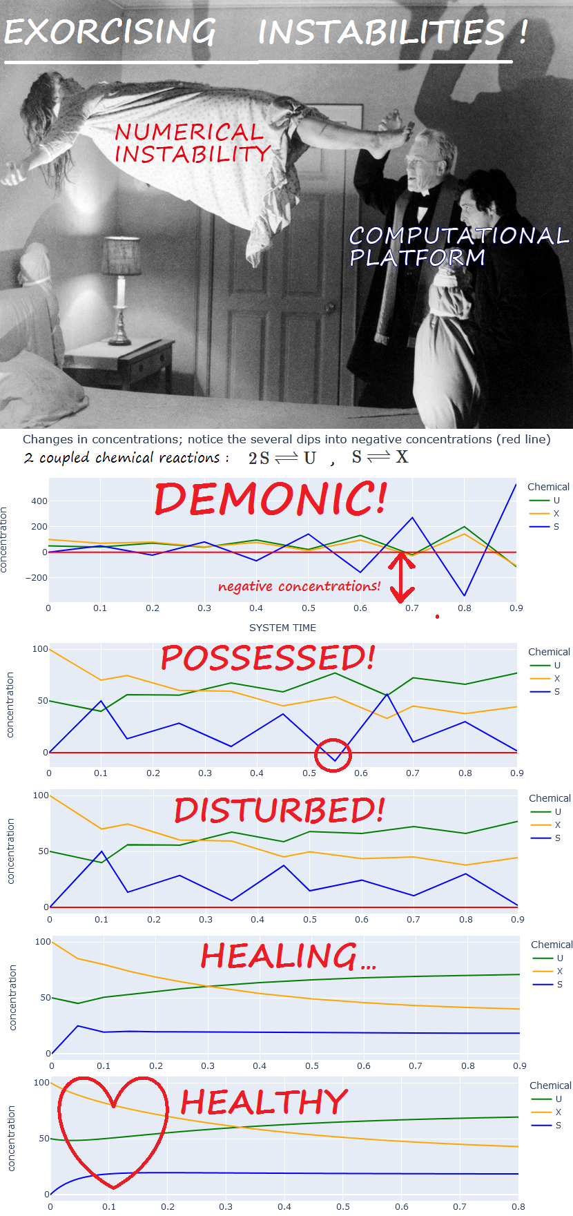
Case study of two coupled reactions: `2 S <-> U` and `S <-> X` (both mostly forward)¶

1st-order kinetics throughout.

LAST REVISED: Nov. 21, 2023 THIS IS AN ARCHIVED EXPERIMENT
(Note: streamlined graphic functions and other improvements were added in later versions of Life123; but this is an ARCHIVED experiment that depends on an old version, as well as depending on special code changes for illustrative purpose. So, this experiment is NOT meant to be run - and for the most part it's not reflecting later changes in the software libraries, though some of the function calls got updated.)

RUN 1 : negative concentrations are detected but otherwise ignored

("DEMONIC" in figure below)

RUN 2 : we restored some, but not all, of the code that had been disabled in Run #1

Negative concentrations from individual reactions are now automatically corrected - but negative concentrations from combined (synergistic) reactions can still slip thru
("POSSESSED" in figure below)

RUN 3 : we restored ALL the code that had been disabled in the earlier runs

Negative concentrations from individual reactions are now automatically corrected - and so are negative concentrations from combined (synergistic) reactions
("DISTURBED" in figure below)

RUN 4 : same as the previous run, but with slightly finer time resolution

("HEALING" in figure below)

For even more accurate solutions - "HEALTHY" in figure below - see the experiment large_time_steps_2

Exorcising Instabilities

IMPORTANT: DO NOT ATTEMPT TO RUN THIS NOTEBOOK!¶

This is a "frozen run" that depends on Life123 code changes for demonstration purposes¶

(a code change that turned off the automatic correction of time steps that lead to negative concentrations.)
If you bypass the execution exit in the first cell, and run the other cells, you WILL NOT REPLICATE the results below!

In [1]:

# To stop the current and subsequent cells: USED TO PREVENT ACCIDENTAL RUNS OF THIS NOTEBOOK!

class StopExecution(Exception):
    def _render_traceback_(self):
        return []

raise StopExecution     # See: https://stackoverflow.com/a/56953105/5478830

The `StopExecution` above is on purpose, TO PREVENT ACCIDENTAL RUNS OF THIS NOTEBOOK!¶

In [ ]:

from src.modules.chemicals.chem_data import ChemData as chem
from src.modules.reactions.reaction_dynamics import ReactionDynamics

import plotly.express as px
import plotly.graph_objects as go

In [3]:

# Initialize the system
chem_data = chem(names=["U", "X", "S"])

# Reaction 2 S <-> U , with 1st-order kinetics for all species (mostly forward)
chem_data.add_reaction(reactants=[(2, "S")], products="U",
                       forward_rate=8., reverse_rate=2.)

# Reaction S <-> X , with 1st-order kinetics for all species (mostly forward)
chem_data.add_reaction(reactants="S", products="X",
                       forward_rate=6., reverse_rate=3.)

chem_data.describe_reactions()

Number of reactions: 2 (at temp. 25 C)
0: 2 S <-> U  (kF = 8 / kR = 2 / Delta_G = -3,436.56 / K = 4) | 1st order in all reactants & products
1: S <-> X  (kF = 6 / kR = 3 / Delta_G = -1,718.28 / K = 2) | 1st order in all reactants & products

RUN 1 : negative concentrations are detected but otherwise ignored ¶

This run required the disabling of multiple software features that detect, and automatically correct, such issues.
It cannot be replicated with current versions of Life123. DO NOT ATTEMPT TO RE-RUN!

In [5]:

dynamics = ReactionDynamics(chem_data=chem_data)
dynamics.set_conc(conc={"U": 50., "X": 100., "S": 0.})
dynamics.describe_state()

SYSTEM STATE at Time t = 0:
3 species:
  Species 0 (U). Conc: 50.0
  Species 1 (X). Conc: 100.0
  Species 2 (S). Conc: 0.0

In [5]:

dynamics.set_diagnostics()       # To save diagnostic information about the call to single_compartment_react()

# ************  DO NOT RUN : Life123 automatically catches and corrects these errors;
#                            this run required a code change for demonstration purposes! 
#                            If you run it, you WILL NOT REPLICATE the results below.
#                            This is meant to be a "frozen run"
dynamics.single_compartment_react(time_step=0.1, stop_time=0.8)

dynamics.explain_time_advance()

+++++++++++ SYSTEM STATE ERROR: FAILED TO CATCH negative concentration upon advancing reactions from system time t=0.45
The computation took 2 extra step(s) - automatically added to prevent negative concentrations
10 total step(s) taken
From time 0 to 0.1, in 1 FULL step of 0.1
From time 0.1 to 0.15, in 1 substep of 0.05 (1/2 of full step)
From time 0.15 to 0.65, in 5 FULL steps of 0.1
From time 0.65 to 0.7, in 1 substep of 0.05 (1/2 of full step)
From time 0.7 to 0.9, in 2 FULL steps of 0.1
(for a grand total of the equivalent of 9 FULL steps)

In [6]:

df = dynamics.get_history()
df

Out[6]:

	SYSTEM TIME	U	X	S	caption
0	0.00	50.000000	100.000000	0.000000	Initial state
1	0.10	40.000000	70.000000	50.000000
2	0.15	56.000000	74.500000	13.500000
3	0.25	55.600000	60.250000	28.550000
4	0.35	67.320000	59.305000	6.055000
5	0.45	58.700000	45.146500	37.453500
6	0.55	76.922800	54.074650	-7.920250
7	0.65	55.202040	33.100105	56.495815
8	0.70	72.280162	45.083834	10.355842
9	0.80	66.108803	37.772189	30.010204
10	0.90	76.895206	44.446655	1.762933

Notice how all concentrations dips into negative values various times!¶

In [8]:

fig0 = dynamics.plot_history(colors=['green', 'orange', 'blue'])   # Prepare, but don't show, the main plot

# Add a second plot, with a horizontal red line at concentration = 0
fig1 = px.line(x=[0,0.9], y=[0,0], color_discrete_sequence = ['red'])

# Combine the plots, and display them   
# (NOTE: streamlined graphic functions were added in later versions, to simplify this kind of plotting; but this is an ARCHIVED experiment -
#        and it's not reflecting those improvements)
all_fig = go.Figure(data=fig0.data + fig1.data, layout = fig0.layout)    # Note that the + is concatenating lists
all_fig.update_layout(title="Changes in concentrations; notice the several dips into negative concentrations (red line)")
all_fig.show()

There are 3 separate scenarios that lead to negative concentrations¶

More information

Scenario 1 : A reaction causes a dip into the negative, and the combined other reactions fail to remedy it¶

Scenario 2 : A reaction causes a dip into the negative, and the other reactions counterbalance it enough to remedy it¶

(though "counterbalanced", this is still regarded as a sign of instability)

Scenario 3 : No single reaction causes any negative concentration, but - combined - they do¶

Example of scenario 1 (all the necessary diagnostic data in the next several rows)
The step from t=0.1 to 0.2 :
[S] is initially 50

Reaction 0 causes a Delta_S of -64.000000 , which would send it into the negative

(leading to message "*** DETECTING NEGATIVE CONCENTRATION in chemical S from reaction 2 S <-> U")

Reaction 1 causes a Delta_S of -9.000000 , which is fine by itself (no error message) but fails to remedy the negative (in fact, makes it worse)

The net result is [S] = 50 -64 -9 = -23 at the final t=0.2
That's what had led to the message "+++ SYSTEM STATE ERROR: FAILED TO CATCH negative concentration upon advancing reactions from system time t=0.1"

Example of scenario 2 (all the necessary diagnostic data in the next several rows)
The step from t=0.4 to 0.5 :
[S] is initially -67.99

Reaction 0 causes a Delta_S of 146.96 , which would remedy the negative when combined with the initial value
Reaction 1 causes a Delta_S of 63.927 , sending [S] into the negative (or, in this case, keeping it into the negative);

(leading to message "*** DETECTING NEGATIVE CONCENTRATION in chemical S from reaction S <-> X")

The net result is [S] = -67.99 +146.96 +63.927 = 142.897 at the final t=0.5
The value is now positive, so there's no SYSTEM STATE ERROR

Example of scenario 3
This scenario doesn't occur in this run, but scroll down to RUN 2 - where it occurs.
An example would be if the initial concentration were 20, and each of the two reactions caused a delta_concentration of -15 ;
combined, they'll bring to concentration to 20 -15 -15 = -10

In [8]:

df

Out[8]:

	SYSTEM TIME	U	X	S	caption
0	0.00	50.000000	100.000000	0.000000	Initial state
1	0.10	40.000000	70.000000	50.000000
2	0.15	56.000000	74.500000	13.500000
3	0.25	55.600000	60.250000	28.550000
4	0.35	67.320000	59.305000	6.055000
5	0.45	58.700000	45.146500	37.453500
6	0.55	76.922800	54.074650	-7.920250
7	0.65	55.202040	33.100105	56.495815
8	0.70	72.280162	45.083834	10.355842
9	0.80	66.108803	37.772189	30.010204
10	0.90	76.895206	44.446655	1.762933

In [9]:

dynamics.get_diagnostic_rxn_data(rxn_index=0)

Reaction:  2 S <-> U

Out[9]:

	TIME	Delta U	Delta S	time_subdivision	delta_time
0	0.00	-10.000000	20.000000	1	0.10
1	0.10	16.000000	-32.000000	1	0.05
2	0.15	-0.400000	0.800000	1	0.10
3	0.25	11.720000	-23.440000	1	0.10
4	0.35	-8.620000	17.240000	1	0.10
5	0.45	18.222800	-36.445600	1	0.10
6	0.55	-21.720760	43.441520	1	0.10
7	0.65	17.078122	-34.156244	1	0.05
8	0.70	-6.171359	12.342717	1	0.10
9	0.80	10.786403	-21.572805	1	0.10

In [10]:

dynamics.get_diagnostic_rxn_data(rxn_index=1)

Reaction:  S <-> X

Out[10]:

	TIME	Delta X	Delta S	reaction	time_subdivision	delta_time
0	0.00	-30.000000	30.000000	1	1	0.10
1	0.10	4.500000	-4.500000	1	1	0.05
2	0.15	-14.250000	14.250000	1	1	0.10
3	0.25	-0.945000	0.945000	1	1	0.10
4	0.35	-14.158500	14.158500	1	1	0.10
5	0.45	8.928150	-8.928150	1	1	0.10
6	0.55	-20.974545	20.974545	1	1	0.10
7	0.65	11.983729	-11.983729	1	1	0.05
8	0.70	-7.311645	7.311645	1	1	0.10
9	0.80	6.674466	-6.674466	1	1	0.10

In [ ]:

##################################################################################

RUN 2 : we restored some, but not all, of the code that had been disabled in Run #1.¶

Negative concentrations from individual reactions are now automatically corrected - but negative concentrations from combined (synergistic) reactions can still slip thru¶

(With the restored code) Life123 automatically detects whenever an individual reaction would cause any chemical concentration to go negative.¶

At that point, it raises an ExcessiveTimeStep exception. That exception gets caught - which results in the following:

the (partial) execution of the last step gets discarded
the step size gets halved
the run automatically resumes from the previous time

Such an automatic detection and remediation eliminates "Scenarios 1 and 2" (see earlier in notebook for definitions) BUT NOT "scenario 3"
IMPORTANT: scenario 3 normally gets caught and remedied, too - but that feature got disabled by a code change in this run, FOR DEMONSTRATION PURPOSES

This run required the disabling of multiple software features that detect, and automatically correct, such issues.
It cannot be replicated with current versions of Life123. DO NOT ATTEMPT TO RE-RUN!

In [4]:

# Same as for Run #1
dynamics = ReactionDynamics(chem_data=chem_data)
dynamics.set_conc(conc={"U": 50., "X": 100., "S": 0.})
dynamics.describe_state()

SYSTEM STATE at Time t = 0:
3 species:
  Species 0 (U). Conc: 50.0
  Species 1 (X). Conc: 100.0
  Species 2 (S). Conc: 0.0

In [6]:

dynamics.set_diagnostics()       # To save diagnostic information about the call to single_compartment_react()

# ************  DO NOT RUN : Life123 automatically catches and corrects these errors;
#                            this run required a code change for demonstration purposes! 
#                            If you run it, you WILL NOT REPLICATE the results below.
#                            This is meant to be a "frozen run"
dynamics.single_compartment_react(time_step=0.1, stop_time=0.8)

dynamics.explain_time_advance()

****** DETECTING NEGATIVE CONCENTRATION in chemical `S` from reaction 2 S <-> U
       [System Time: 0.1 : Baseline value: 50 ; delta conc: -64]
       IGNORING AND CONTINUING (for demonstration purposes)
+++++++++++ SYSTEM STATE ERROR: FAILED TO CATCH negative concentration upon advancing reactions from system time t=0.1
****** DETECTING NEGATIVE CONCENTRATION in chemical `S` from reaction 2 S <-> U
       [System Time: 0.3 : Baseline value: 80.1 ; delta conc: -112.48]
       IGNORING AND CONTINUING (for demonstration purposes)
+++++++++++ SYSTEM STATE ERROR: FAILED TO CATCH negative concentration upon advancing reactions from system time t=0.3
****** DETECTING NEGATIVE CONCENTRATION in chemical `S` from reaction S <-> X
       [System Time: 0.4 : Baseline value: -67.99 ; delta conc: 63.927]
       IGNORING AND CONTINUING (for demonstration purposes)
****** DETECTING NEGATIVE CONCENTRATION in chemical `S` from reaction 2 S <-> U
       [System Time: 0.5 : Baseline value: 142.9 ; delta conc: -219.85]
       IGNORING AND CONTINUING (for demonstration purposes)
+++++++++++ SYSTEM STATE ERROR: FAILED TO CATCH negative concentration upon advancing reactions from system time t=0.5
****** DETECTING NEGATIVE CONCENTRATION in chemical `U` from reaction 2 S <-> U
       [System Time: 0.6 : Baseline value: 131.89 ; delta conc: -153.37]
       IGNORING AND CONTINUING (for demonstration purposes)
****** DETECTING NEGATIVE CONCENTRATION in chemical `S` from reaction S <-> X
       [System Time: 0.6 : Baseline value: -158.74 ; delta conc: 123.73]
       IGNORING AND CONTINUING (for demonstration purposes)
****** DETECTING NEGATIVE CONCENTRATION in chemical `X` from reaction S <-> X
       [System Time: 0.6 : Baseline value: 94.966 ; delta conc: -123.73]
       IGNORING AND CONTINUING (for demonstration purposes)
+++++++++++ SYSTEM STATE ERROR: FAILED TO CATCH negative concentration upon advancing reactions from system time t=0.6
****** DETECTING NEGATIVE CONCENTRATION in chemical `S` from reaction 2 S <-> U
       [System Time: 0.7 : Baseline value: 271.73 ; delta conc: -443.36]
       IGNORING AND CONTINUING (for demonstration purposes)
+++++++++++ SYSTEM STATE ERROR: FAILED TO CATCH negative concentration upon advancing reactions from system time t=0.7
****** DETECTING NEGATIVE CONCENTRATION in chemical `U` from reaction 2 S <-> U
       [System Time: 0.8 : Baseline value: 200.2 ; delta conc: -314.68]
       IGNORING AND CONTINUING (for demonstration purposes)
****** DETECTING NEGATIVE CONCENTRATION in chemical `S` from reaction S <-> X
       [System Time: 0.8 : Baseline value: -343.3 ; delta conc: 248.85]
       IGNORING AND CONTINUING (for demonstration purposes)
****** DETECTING NEGATIVE CONCENTRATION in chemical `X` from reaction S <-> X
       [System Time: 0.8 : Baseline value: 142.9 ; delta conc: -248.85]
       IGNORING AND CONTINUING (for demonstration purposes)
+++++++++++ SYSTEM STATE ERROR: FAILED TO CATCH negative concentration upon advancing reactions from system time t=0.8
9 total step(s) taken
From time 0 to 0.9, in 9 FULL steps of 0.1
(for a grand total of the equivalent of 9 FULL steps)

Notice how the system automatically temporarily slowed down from the requested time step of 0.1 at t=0.1 and again at t=0.65¶

Those actions intercepted, and automatically remedied, some - but NOT all - of the negative concentrations (explained below in the notebook.)
We now took a total of 10 steps, instead of the 9 ones of Run #1

In [6]:

df = dynamics.get_history()
df

Out[6]:

	SYSTEM TIME	U	X	S	caption
0	0.00	50.000000	100.000000	0.000000	Initial state
1	0.10	40.000000	70.000000	50.000000
2	0.15	56.000000	74.500000	13.500000
3	0.25	55.600000	60.250000	28.550000
4	0.35	67.320000	59.305000	6.055000
5	0.45	58.700000	45.146500	37.453500
6	0.50	67.811400	49.610575	14.766625
7	0.60	66.062420	43.587378	24.287783
8	0.70	72.280162	45.083834	10.355842
9	0.80	66.108803	37.772189	30.010204
10	0.90	76.895206	44.446655	1.762933

Notice how [S] dips into negative values at t=0.55!¶

But all the multitude of other negative dips we had in Run #1 are now gone :)

In [7]:

fig0 = dynamics.plot_history(colors=['green', 'orange', 'blue'])   # Prepare, but don't show, the main plot

# Add a second plot, with a horizontal red line at concentration = 0
fig1 = px.line(x=[0,0.9], y=[0,0], color_discrete_sequence = ['red'])

# Combine the plots, and display them
all_fig = go.Figure(data=fig0.data + fig1.data, layout = fig0.layout)    # Note that the + is concatenating lists
all_fig.update_layout(title="Changes in concentrations; notice how S dips into negative concentrations (red line) at t=0.55")
all_fig.show()

With this partially-restored functionality, we're averting what we called "scenarios 1 and 2" earlier in the notebook - but are still afflicted by "scenario 3" (no single reaction causes any negative concentration, but - combined - they do)¶

That's exactly what happens to [S] at t=0.55 (all the necessary diagnostic data in the next few rows)
The step from t=0.45 to 0.55 :
[S] is initially 37.453500

Reaction 0 causes a Delta_S of -36.445600 , which by itself would cause no problem
Reaction 1 causes a Delta_S of -8.928150 , by itself would cause no problem - but leads to a negative value when combined with reaction 0!

The net result is [S] = 37.453500 -36.445600 -8.928150 = -7.92025 at the final t=0.55
That's what had led to the message "+++ SYSTEM STATE ERROR: FAILED TO CATCH negative concentration upon advancing reactions from system time t=0.45"

In [9]:

df

Out[9]:

	SYSTEM TIME	U	X	S	caption
0	0.0	50.000000	100.000000	0.000000	Initial state
1	0.1	40.000000	70.000000	50.000000
2	0.2	72.000000	79.000000	-23.000000
3	0.3	39.200000	41.500000	80.100000
4	0.4	95.440000	77.110000	-67.990000
5	0.5	21.960000	13.183000	142.897000
6	0.6	131.885600	94.966300	-158.737500
7	0.7	-21.481520	-28.766090	271.729130
8	0.8	200.198088	142.901215	-343.297391
9	0.9	-114.479442	-105.947584	534.906469

In [10]:

dynamics.get_diagnostic_rxn_data(rxn_index=0)

Reaction:  2 S <-> U

Out[10]:

	TIME	Delta U	Delta S	time_subdivision	delta_time
0	0.0	-10.000000	20.000000	1	0.1
1	0.1	32.000000	-64.000000	1	0.1
2	0.2	-32.800000	65.600000	1	0.1
3	0.3	56.240000	-112.480000	1	0.1
4	0.4	-73.480000	146.960000	1	0.1
5	0.5	109.925600	-219.851200	1	0.1
6	0.6	-153.367120	306.734240	1	0.1
7	0.7	221.679608	-443.359216	1	0.1
8	0.8	-314.677530	629.355061	1	0.1

In [11]:

dynamics.get_diagnostic_rxn_data(rxn_index=1)

Reaction:  S <-> X

Out[11]:

	TIME	Delta X	Delta S	reaction	time_subdivision	delta_time
0	0.0	-30.000000	30.000000	1	1	0.1
1	0.1	9.000000	-9.000000	1	1	0.1
2	0.2	-37.500000	37.500000	1	1	0.1
3	0.3	35.610000	-35.610000	1	1	0.1
4	0.4	-63.927000	63.927000	1	1	0.1
5	0.5	81.783300	-81.783300	1	1	0.1
6	0.6	-123.732390	123.732390	1	1	0.1
7	0.7	171.667305	-171.667305	1	1	0.1
8	0.8	-248.848799	248.848799	1	1	0.1

In [ ]:

##################################################################################

RUN 3 : we restored ALL the code that had been disabled in the earlier runs.¶

Negative concentrations from individual reactions are now automatically corrected - and so are negative concentrations from combined (synergistic) reactions¶

(With the restored code) Life123 automatically detects whenever any chemical concentration goes negative from any cause.¶

At that point, it raises an ExcessiveTimeStep exception. That exception gets caught - which results in the following:

the (partial) execution of the last step gets discarded
the step size gets halved
the run automatically resumes from the previous time

In [4]:

# Same as for the previous runs
dynamics = ReactionDynamics(chem_data=chem_data)
dynamics.set_conc(conc={"U": 50., "X": 100., "S": 0.})
dynamics.describe_state()

SYSTEM STATE at Time t = 0:
3 species:
  Species 0 (U). Conc: 50.0
  Species 1 (X). Conc: 100.0
  Species 2 (S). Conc: 0.0

In [5]:

dynamics.set_diagnostics()       # To save diagnostic information about the call to single_compartment_react()

dynamics.single_compartment_react(time_step=0.1, stop_time=0.8)

dynamics.explain_time_advance()

******** CAUTION: negative concentration in chemical `S` (resulting from reaction 2 S <-> U)
         upon advancing from system time t=0.1 [Baseline value: 50 ; delta conc: -64]
         It will be AUTOMATICALLY CORRECTED with a reduction in the time step size
******** CAUTION: negative concentration resulting from the combined effect of multiple reactions, upon advancing reactions from system time t=0.45
         It will be AUTOMATICALLY CORRECTED with a reduction in the time step size
The computation took 2 extra step(s) - automatically added to prevent negative concentrations
10 total step(s) taken
From time 0 to 0.1, in 1 FULL step of 0.1
From time 0.1 to 0.15, in 1 substep of 0.05 (1/2 of full step)
From time 0.15 to 0.45, in 3 FULL steps of 0.1
From time 0.45 to 0.5, in 1 substep of 0.05 (1/2 of full step)
From time 0.5 to 0.9, in 4 FULL steps of 0.1
(for a grand total of the equivalent of 9 FULL steps)

Notice how the system automatically temporarily slowed down from the requested time step of 0.1 at t=0.1 and again at t=0.45¶

Those actions intercepted, and automatically remedied, ALL the negative concentrations, whether caused by any single reaction, or by the cumulative effect of multiple ones.
We now took a total of 10 steps, instead of the 9 ones of Run #1

In [10]:

df = dynamics.get_history()
df

Out[10]:

	SYSTEM TIME	U	X	S	caption
0	0.00	50.000000	100.000000	0.000000	Initial state
1	0.05	45.000000	85.000000	25.000000	Interm. step, due to the fast rxns: [0, 1]
2	0.10	50.500000	79.750000	19.250000
3	0.15	53.150000	73.562500	20.137500	Interm. step, due to the fast rxns: [0, 1]
4	0.20	55.890000	68.569375	19.650625
5	0.25	58.161250	64.179156	19.498344	Interm. step, due to the fast rxns: [0, 1]
6	0.30	60.144463	60.401786	19.309289
7	0.40	63.563001	53.866824	19.007174
8	0.50	66.056140	49.111081	18.776639
9	0.60	67.866223	45.643740	18.623814
10	0.70	69.192029	43.124906	18.491035
11	0.80	70.146452	41.282055	18.425042
12	0.90	70.857195	39.952464	18.333147

Notice how negative concentrations are no longer seen anywhere :)¶

In [7]:

fig0 = dynamics.plot_history(colors=['green', 'orange', 'blue'])   # Prepare, but don't show, the main plot

# Add a second plot, with a horizontal red line at concentration = 0
fig1 = px.line(x=[0,0.9], y=[0,0], color_discrete_sequence = ['red'])

# Combine the plots, and display them
all_fig = go.Figure(data=fig0.data + fig1.data, layout = fig0.layout)    # Note that the + is concatenating lists
all_fig.update_layout(title="Changes in concentrations; notice negative concentrations are totally absent now")
all_fig.show()

With the completely-restored functionality, we're averting what we called "scenarios 1, 2 and 3" earlier in the notebook :)¶

In [ ]:

##################################################################################

RUN 4 : same as the previous run, but with slightly finer time resolution ¶

In run 3, we demonstrated catching - and resolving - all cases of negative concentrations that would slip in if it weren't for Life123's detection and automatic remediation. But we still have a lot of instability, especially in [S].

A slight improvement in the time steps will make a profound difference in this run

In [8]:

# Same as for the previous runs
dynamics = ReactionDynamics(chem_data=chem_data)
dynamics.set_conc(conc={"U": 50., "X": 100., "S": 0.})
dynamics.describe_state()

SYSTEM STATE at Time t = 0:
3 species:
  Species 0 (U). Conc: 50.0
  Species 1 (X). Conc: 100.0
  Species 2 (S). Conc: 0.0

Rather than decreasing (for the whole run) the time step of 0.1, we'll simply opt to AUTOMATICALLY take 2 substeps whenever any of the reactions are "fast changing" based on a threshold we provide¶

In [9]:

dynamics.set_diagnostics()       # To save diagnostic information about the call to single_compartment_react()

dynamics.single_compartment_react(time_step=0.1, stop_time=0.8, 
                                  dynamic_substeps=2, abs_fast_threshold=80.0)

dynamics.explain_time_advance()

single_compartment_react(): setting rel_fast_threshold to 800.0
9 total step(s) taken
From time 0 to 0.3, in 6 substeps of 0.05 (each 1/2 of full step)
From time 0.3 to 0.9, in 6 FULL steps of 0.1
(for a grand total of the equivalent of 9 FULL steps)

Note how the system automatically splits the time steps into substeps for up to t=0.3¶

that's when most of the change is occurring

In [7]:

df = dynamics.get_history()
df

Out[7]:

	SYSTEM TIME	U	X	S	caption
0	0.0	50.000000	100.000000	0.000000	Initial state
1	0.1	40.000000	70.000000	50.000000
2	0.2	72.000000	79.000000	-23.000000
3	0.3	39.200000	41.500000	80.100000
4	0.4	95.440000	77.110000	-67.990000
5	0.5	21.960000	13.183000	142.897000
6	0.6	131.885600	94.966300	-158.737500
7	0.7	-21.481520	-28.766090	271.729130
8	0.8	200.198088	142.901215	-343.297391
9	0.9	-114.479442	-105.947584	534.906469

In [ ]:

dynamics.plot_history(colors=['green', 'orange', 'blue'])

The resolution is still coarse, especially up to t=0.1, but all the instability is gone :)¶

Note: For even more accurate solutions, see the experiment `large_time_steps_2`¶

In [ ]:

Tour of Life123's process of automatic detection - and stepsize reduction - in case any concentration goes negative¶

Case study of two coupled reactions: 2 S <-> U and S <-> X (both mostly forward)¶

IMPORTANT: DO NOT ATTEMPT TO RUN THIS NOTEBOOK!¶

This is a "frozen run" that depends on Life123 code changes for demonstration purposes¶

The StopExecution above is on purpose, TO PREVENT ACCIDENTAL RUNS OF THIS NOTEBOOK!¶

RUN 1 : negative concentrations are detected but otherwise ignored¶

Notice how all concentrations dips into negative values various times!¶

There are 3 separate scenarios that lead to negative concentrations¶

Scenario 1 : A reaction causes a dip into the negative, and the combined other reactions fail to remedy it¶

Scenario 2 : A reaction causes a dip into the negative, and the other reactions counterbalance it enough to remedy it¶

Scenario 3 : No single reaction causes any negative concentration, but - combined - they do¶

RUN 2 : we restored some, but not all, of the code that had been disabled in Run #1.¶

Negative concentrations from individual reactions are now automatically corrected - but negative concentrations from combined (synergistic) reactions can still slip thru¶

(With the restored code) Life123 automatically detects whenever an individual reaction would cause any chemical concentration to go negative.¶

Notice how the system automatically temporarily slowed down from the requested time step of 0.1 at t=0.1 and again at t=0.65¶

Notice how [S] dips into negative values at t=0.55!¶

With this partially-restored functionality, we're averting what we called "scenarios 1 and 2" earlier in the notebook - but are still afflicted by "scenario 3" (no single reaction causes any negative concentration, but - combined - they do)¶

RUN 3 : we restored ALL the code that had been disabled in the earlier runs.¶

Negative concentrations from individual reactions are now automatically corrected - and so are negative concentrations from combined (synergistic) reactions¶

(With the restored code) Life123 automatically detects whenever any chemical concentration goes negative from any cause.¶

Notice how the system automatically temporarily slowed down from the requested time step of 0.1 at t=0.1 and again at t=0.45¶

Notice how negative concentrations are no longer seen anywhere :)¶

With the completely-restored functionality, we're averting what we called "scenarios 1, 2 and 3" earlier in the notebook :)¶

RUN 4 : same as the previous run, but with slightly finer time resolution¶

Rather than decreasing (for the whole run) the time step of 0.1, we'll simply opt to AUTOMATICALLY take 2 substeps whenever any of the reactions are "fast changing" based on a threshold we provide¶

Note how the system automatically splits the time steps into substeps for up to t=0.3¶

The resolution is still coarse, especially up to t=0.1, but all the instability is gone :)¶

Note: For even more accurate solutions, see the experiment large_time_steps_2¶

Case study of two coupled reactions: `2 S <-> U` and `S <-> X` (both mostly forward)¶

The `StopExecution` above is on purpose, TO PREVENT ACCIDENTAL RUNS OF THIS NOTEBOOK!¶

RUN 1 : negative concentrations are detected but otherwise ignored ¶

RUN 4 : same as the previous run, but with slightly finer time resolution ¶

Note: For even more accurate solutions, see the experiment `large_time_steps_2`¶