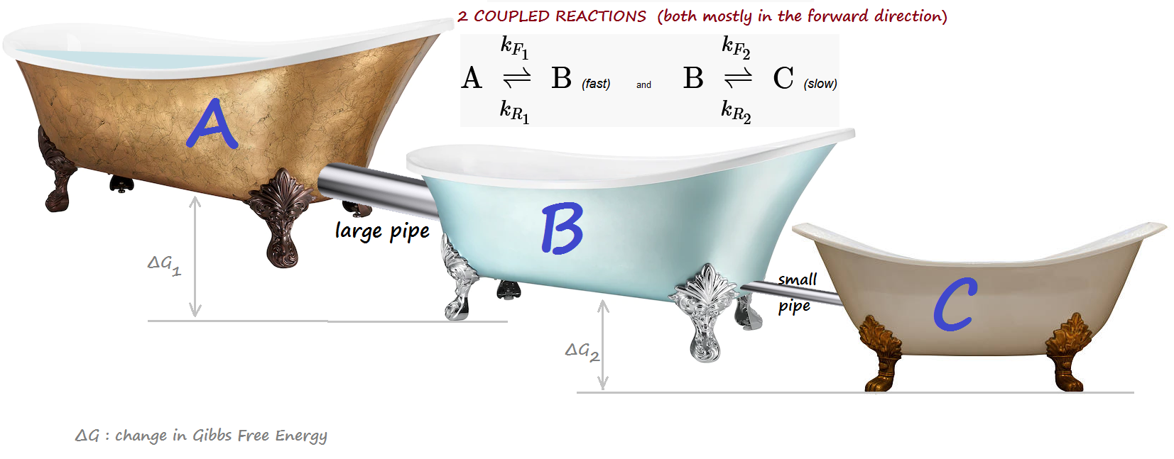
2 COUPLED reactions of different speeds, forming a "cascade":¶

`A <-> B` (fast) and `B <-> C` (slow)¶

Taken to equilibrium. Both reactions are mostly forward. All 1st order.
The concentration of the intermediate product B manifests 1 oscillation (transient "overshoot")

Adaptive variable time resolution is used, with extensive diagnostics, and finally compared to a new run using fixed time intervals, with the same initial data.

In part2, some diagnotic insight is explored.
In part3, two identical runs ("adaptive variable steps" and "fixed small steps") are compared.

LAST REVISED: May 27, 2024 (using v. 1.0beta32)

Bathtub analogy:¶

A is initially full, while B and C are empty.
Tubs are progressively lower (reactions are mostly forward.)
A BIG pipe connects A and B: fast kinetics. A small pipe connects B and C: slow kinetics.

INTUITION: B, unable to quickly drain into C while at the same time being blasted by a hefty inflow from A,
will experience a transient surge, in excess of its final equilibrium level.

Compare with the final reaction plot (the orange line is B)

2 Coupled Reactions

In [1]:

import set_path      # Importing this module will add the project's home directory to sys.path

Added 'D:\Docs\- MY CODE\BioSimulations\life123-Win7' to sys.path

In [2]:

from experiments.get_notebook_info import get_notebook_basename

from src.modules.chemicals.chem_data import ChemData
from src.modules.reactions.reaction_dynamics import ReactionDynamics
from src.modules.visualization.plotly_helper import PlotlyHelper

from src.modules.visualization.graphic_log import GraphicLog

In [3]:

# Initialize the HTML logging (for the graphics)
log_file = get_notebook_basename() + ".log.htm"    # Use the notebook base filename for the log file

# Set up the use of some specified graphic (Vue) components
GraphicLog.config(filename=log_file,
                  components=["vue_cytoscape_2"],
                  extra_js="https://cdnjs.cloudflare.com/ajax/libs/cytoscape/3.21.2/cytoscape.umd.js")

-> Output will be LOGGED into the file 'cascade_1.log.htm'

Initialize the System¶

Specify the chemicals and the reactions

In [4]:

# Instantiate the simulator and specify the chemicals
chem = ChemData(names=["A", "B", "C"])

# Reaction A <-> B (fast)
chem.add_reaction(reactants=["A"], products=["B"],
                       forward_rate=64., reverse_rate=8.) 

# Reaction B <-> C (slow)
chem.add_reaction(reactants=["B"], products=["C"],
                       forward_rate=12., reverse_rate=2.) 

print("Number of reactions: ", chem.number_of_reactions())

Number of reactions:  2

In [5]:

chem.describe_reactions()

Number of reactions: 2 (at temp. 25 C)
0: A <-> B  (kF = 64 / kR = 8 / delta_G = -5,154.8 / K = 8) | 1st order in all reactants & products
1: B <-> C  (kF = 12 / kR = 2 / delta_G = -4,441.7 / K = 6) | 1st order in all reactants & products
Set of chemicals involved in the above reactions: {'A', 'C', 'B'}

In [6]:

# Send a plot of the network of reactions to the HTML log file
chem.plot_reaction_network("vue_cytoscape_2")

[GRAPHIC ELEMENT SENT TO LOG FILE `cascade_1.log.htm`]

Run the simulation¶

In [7]:

dynamics = ReactionDynamics(chem_data=chem, preset="fast")

dynamics.set_conc([50., 0, 0.], snapshot=True) # Set the initial concentrations of all the chemicals, in their index order
dynamics.describe_state()

SYSTEM STATE at Time t = 0:
3 species:
  Species 0 (A). Conc: 50.0
  Species 1 (B). Conc: 0.0
  Species 2 (C). Conc: 0.0
Set of chemicals involved in reactions: {'A', 'C', 'B'}

In [8]:

dynamics.get_history()

Out[8]:

	SYSTEM TIME	A	B	C	caption
0	0.0	50.0	0.0	0.0	Initialized state

Run the reaction¶

In [9]:

dynamics.set_diagnostics()         # To save diagnostic information about the call to single_compartment_react()

dynamics.single_compartment_react(initial_step=0.02, reaction_duration=0.4,
                                  snapshots={"initial_caption": "1st reaction step",
                                             "final_caption": "last reaction step"},
                                  variable_steps=True, explain_variable_steps=False)

*** CAUTION: negative concentration in chemical `A` in step starting at t=0.  It will be AUTOMATICALLY CORRECTED with a reduction in time step size, as follows:
    INFO: the tentative time step (0.02) leads to a NEGATIVE concentration of `A` from reaction A <-> B (rxn # 0): 
      Baseline value: 50 ; delta conc: -64
      -> will backtrack, and re-do step with a SMALLER delta time, multiplied by 0.5 (set to 0.01) [Step started at t=0, and will rewind there]
* INFO: the tentative time step (0.01) leads to a least one norm value > its ABORT threshold:
      -> will backtrack, and re-do step with a SMALLER delta time, multiplied by 0.6 (set to 0.006) [Step started at t=0, and will rewind there]
* INFO: the tentative time step (0.006) leads to a least one norm value > its ABORT threshold:
      -> will backtrack, and re-do step with a SMALLER delta time, multiplied by 0.6 (set to 0.0036) [Step started at t=0, and will rewind there]
* INFO: the tentative time step (0.0036) leads to a least one norm value > its ABORT threshold:
      -> will backtrack, and re-do step with a SMALLER delta time, multiplied by 0.6 (set to 0.00216) [Step started at t=0, and will rewind there]
* INFO: the tentative time step (0.00216) leads to a least one norm value > its ABORT threshold:
      -> will backtrack, and re-do step with a SMALLER delta time, multiplied by 0.6 (set to 0.001296) [Step started at t=0, and will rewind there]
* INFO: the tentative time step (0.001296) leads to a least one norm value > its ABORT threshold:
      -> will backtrack, and re-do step with a SMALLER delta time, multiplied by 0.6 (set to 0.0007776) [Step started at t=0, and will rewind there]
Some steps were backtracked and re-done, to prevent negative concentrations or excessively large concentration changes
48 total step(s) taken

Plots of changes of concentration with time ¶

Notice the variable time steps (vertical dashed lines)

In [10]:

dynamics.plot_history(title="Coupled reactions A <-> B and B <-> C",
                      colors=['blue', 'orange', 'green'], show_intervals=True)

In [11]:

dynamics.curve_intersect("A", "B", t_start=0, t_end=0.05)

Out[11]:

(0.011857732428358053, 24.047031609298816)

In [12]:

dynamics.curve_intersect("A", "C", t_start=0, t_end=0.05)

Out[12]:

(0.031934885008449314, 8.852813807230596)

In [13]:

dynamics.curve_intersect("B", "C", t_start=0.05, t_end=0.1)

Out[13]:

(0.07740303497735611, 23.285274847029168)

In [14]:

dynamics.get_history()

Out[14]:

	SYSTEM TIME	A	B	C	caption
0	0.000000	50.000000	0.000000	0.000000	Initialized state
1	0.000778	47.511680	2.488320	0.000000	1st reaction step
2	0.001400	45.632475	4.348950	0.018575
3	0.002022	43.837347	6.111636	0.051017
4	0.002519	42.465438	7.447097	0.087465
5	0.003017	41.142542	8.725606	0.131851
6	0.003515	39.866871	9.949300	0.183829
7	0.004012	38.636703	11.120234	0.243063
8	0.004510	37.450378	12.240391	0.309231
9	0.005008	36.306298	13.311680	0.382022
10	0.005505	35.202922	14.335939	0.461139
11	0.006003	34.138767	15.314939	0.546294
12	0.006501	33.112404	16.250386	0.637210
13	0.006998	32.122455	17.143922	0.733623
14	0.007496	31.167595	17.997130	0.835276
15	0.008243	29.786018	19.218736	0.995246
16	0.008989	28.477742	20.356337	1.165921
17	0.009736	27.238764	21.414705	1.346531
18	0.010482	26.065300	22.398347	1.536353
19	0.011602	24.398010	23.768113	1.833877
20	0.012722	22.862474	24.988386	2.149140
21	0.013841	21.447911	26.071994	2.480095
22	0.014961	20.144428	27.030704	2.824868
23	0.016641	18.342204	28.297603	3.360193
24	0.018320	16.750734	29.330012	3.919255
25	0.020000	15.344212	30.158542	4.497247
26	0.022519	13.477920	31.135708	5.386372
27	0.025039	11.932250	31.767190	6.300559
28	0.027558	10.648537	32.122231	7.229232
29	0.031337	9.044186	32.324491	8.631323
30	0.035116	7.833986	32.134026	10.031989
31	0.038896	6.910732	31.675838	11.413430
32	0.044564	5.840026	30.721211	13.438763
33	0.050233	5.114478	29.509327	15.376196
34	0.058736	4.338557	27.535703	18.125740
35	0.065538	3.948219	25.924919	20.126862
36	0.075742	3.486129	23.623393	22.890478
37	0.083905	3.207568	21.961627	24.830805
38	0.096149	2.845240	19.705148	27.449612
39	0.105945	2.605699	18.166190	29.228112
40	0.120638	2.290745	16.137006	31.572249
41	0.135332	2.033442	14.476842	33.489716
42	0.157371	1.717708	12.439976	35.842316
43	0.179411	1.488195	10.959299	37.552505
44	0.212471	1.237929	9.344771	39.417300
45	0.245531	1.090175	8.391543	40.518282
46	0.295121	0.959315	7.547371	41.493315
47	0.369506	0.883653	7.059061	42.057286
48	0.481083	0.874584	7.001835	42.123581	last reaction step

In [15]:

dynamics.explain_time_advance()

From time 0 to 0.0007776, in 1 step of 0.000778
From time 0.0007776 to 0.002022, in 2 steps of 0.000622
From time 0.002022 to 0.007496, in 11 steps of 0.000498
From time 0.007496 to 0.01048, in 4 steps of 0.000746
From time 0.01048 to 0.01496, in 4 steps of 0.00112
From time 0.01496 to 0.02, in 3 steps of 0.00168
From time 0.02 to 0.02756, in 3 steps of 0.00252
From time 0.02756 to 0.0389, in 3 steps of 0.00378
From time 0.0389 to 0.05023, in 2 steps of 0.00567
From time 0.05023 to 0.05874, in 1 step of 0.0085
From time 0.05874 to 0.06554, in 1 step of 0.0068
From time 0.06554 to 0.07574, in 1 step of 0.0102
From time 0.07574 to 0.08391, in 1 step of 0.00816
From time 0.08391 to 0.09615, in 1 step of 0.0122
From time 0.09615 to 0.1059, in 1 step of 0.0098
From time 0.1059 to 0.1353, in 2 steps of 0.0147
From time 0.1353 to 0.1794, in 2 steps of 0.022
From time 0.1794 to 0.2455, in 2 steps of 0.0331
From time 0.2455 to 0.2951, in 1 step of 0.0496
From time 0.2951 to 0.3695, in 1 step of 0.0744
From time 0.3695 to 0.4811, in 1 step of 0.112
(48 steps total)

Check the final equilibrium¶

In [16]:

# Verify that all the reactions have reached equilibrium
dynamics.is_in_equilibrium()

0: A <-> B
Final concentrations: [A] = 0.8746 ; [B] = 7.002
1. Ratio of reactant/product concentrations, adjusted for reaction orders: 8.0059
    Formula used:  [B] / [A]
2. Ratio of forward/reverse reaction rates: 8.0
Discrepancy between the two values: 0.07378 %
Reaction IS in equilibrium (within 1% tolerance)

1: B <-> C
Final concentrations: [C] = 42.12 ; [B] = 7.002
1. Ratio of reactant/product concentrations, adjusted for reaction orders: 6.01608
    Formula used:  [C] / [B]
2. Ratio of forward/reverse reaction rates: 6.0
Discrepancy between the two values: 0.268 %
Reaction IS in equilibrium (within 1% tolerance)

Out[16]:

True

Let's look at the final concentrations of `A` and `C` (i.e., the reactant and product of the composite reaction)¶

In [17]:

A_final = dynamics.get_chem_conc("A")
A_final

Out[17]:

0.8745841244150234

In [18]:

C_final = dynamics.get_chem_conc("C")
C_final

Out[18]:

42.123581082850514

Their ratio:¶

In [19]:

C_final / A_final

Out[19]:

48.16412727709344

As expected the equilibrium constant for the overall reaction `A <-> C` (approx. 48) is indeed the product of the equilibrium constants of the two elementary reactions (K = 8 and K = 6, respectively) that we saw earlier.¶

In [ ]:

PART 2 - DIAGNOSTIC INSIGHT¶

Perform some verification

Take a peek at the diagnostic data saved during the earlier reaction simulation¶

In [20]:

# Concentration increments due to reaction 0 (A <-> B)
# Note that [C] is not affected
dynamics.get_diagnostic_rxn_data(rxn_index=0)

Reaction:  A <-> B

Out[20]:

	START_TIME	Delta A	Delta B	Delta C	time_step	caption
0	0.000000	NaN	NaN	NaN	0.020000	aborted: neg. conc. in `A`
1	0.000000	-32.000000	32.000000	0.0	0.010000	aborted: excessive norm value(s)
2	0.000000	-19.200000	19.200000	0.0	0.006000	aborted: excessive norm value(s)
3	0.000000	-11.520000	11.520000	0.0	0.003600	aborted: excessive norm value(s)
4	0.000000	-6.912000	6.912000	0.0	0.002160	aborted: excessive norm value(s)
5	0.000000	-4.147200	4.147200	0.0	0.001296	aborted: excessive norm value(s)
6	0.000000	-2.488320	2.488320	0.0	0.000778
7	0.000778	-1.879205	1.879205	0.0	0.000622
8	0.001400	-1.795128	1.795128	0.0	0.000622
9	0.002022	-1.371909	1.371909	0.0	0.000498
10	0.002519	-1.322896	1.322896	0.0	0.000498
11	0.003017	-1.275671	1.275671	0.0	0.000498
12	0.003515	-1.230168	1.230168	0.0	0.000498
13	0.004012	-1.186325	1.186325	0.0	0.000498
14	0.004510	-1.144080	1.144080	0.0	0.000498
15	0.005008	-1.103376	1.103376	0.0	0.000498
16	0.005505	-1.064155	1.064155	0.0	0.000498
17	0.006003	-1.026363	1.026363	0.0	0.000498
18	0.006501	-0.989949	0.989949	0.0	0.000498
19	0.006998	-0.954861	0.954861	0.0	0.000498
20	0.007496	-1.381577	1.381577	0.0	0.000746
21	0.008243	-1.308275	1.308275	0.0	0.000746
22	0.008989	-1.238978	1.238978	0.0	0.000746
23	0.009736	-1.173464	1.173464	0.0	0.000746
24	0.010482	-1.667290	1.667290	0.0	0.001120
25	0.011602	-1.535536	1.535536	0.0	0.001120
26	0.012722	-1.414563	1.414563	0.0	0.001120
27	0.013841	-1.303483	1.303483	0.0	0.001120
28	0.014961	-1.802224	1.802224	0.0	0.001680
29	0.016641	-1.591470	1.591470	0.0	0.001680
30	0.018320	-1.406522	1.406522	0.0	0.001680
31	0.020000	-1.866292	1.866292	0.0	0.002519
32	0.022519	-1.545670	1.545670	0.0	0.002519
33	0.025039	-1.283713	1.283713	0.0	0.002519
34	0.027558	-1.604351	1.604351	0.0	0.003779
35	0.031337	-1.210200	1.210200	0.0	0.003779
36	0.035116	-0.923254	0.923254	0.0	0.003779
37	0.038896	-1.070706	1.070706	0.0	0.005669
38	0.044564	-0.725549	0.725549	0.0	0.005669
39	0.050233	-0.775920	0.775920	0.0	0.008503
40	0.058736	-0.390338	0.390338	0.0	0.006802
41	0.065538	-0.462090	0.462090	0.0	0.010204
42	0.075742	-0.278561	0.278561	0.0	0.008163
43	0.083905	-0.362328	0.362328	0.0	0.012244
44	0.096149	-0.239541	0.239541	0.0	0.009796
45	0.105945	-0.314953	0.314953	0.0	0.014693
46	0.120638	-0.257304	0.257304	0.0	0.014693
47	0.135332	-0.315733	0.315733	0.0	0.022040
48	0.157371	-0.229513	0.229513	0.0	0.022040
49	0.179411	-0.250266	0.250266	0.0	0.033060
50	0.212471	-0.147754	0.147754	0.0	0.033060
51	0.245531	-0.130860	0.130860	0.0	0.049590
52	0.295121	-0.075662	0.075662	0.0	0.074385
53	0.369506	-0.009068	0.009068	0.0	0.111577

In [21]:

# Concentration increments due to reaction 1 (B <-> C)
# Note that [A] is not affected.  
# Also notice that the 0-th row from the A <-> B reaction isn't seen here, because that step was aborted
# early on, before even getting to THIS reaction
dynamics.get_diagnostic_rxn_data(rxn_index=1)

Reaction:  B <-> C

Out[21]:

	START_TIME	Delta B	Delta C	time_step	caption
0	0.000000	0.000000	0.000000	0.010000	aborted: excessive norm value(s)
1	0.000000	0.000000	0.000000	0.006000	aborted: excessive norm value(s)
2	0.000000	0.000000	0.000000	0.003600	aborted: excessive norm value(s)
3	0.000000	0.000000	0.000000	0.002160	aborted: excessive norm value(s)
4	0.000000	0.000000	0.000000	0.001296	aborted: excessive norm value(s)
5	0.000000	0.000000	0.000000	0.000778
6	0.000778	-0.018575	0.018575	0.000622
7	0.001400	-0.032442	0.032442	0.000622
8	0.002022	-0.036448	0.036448	0.000498
9	0.002519	-0.044387	0.044387	0.000498
10	0.003017	-0.051978	0.051978	0.000498
11	0.003515	-0.059234	0.059234	0.000498
12	0.004012	-0.066168	0.066168	0.000498
13	0.004510	-0.072791	0.072791	0.000498
14	0.005008	-0.079117	0.079117	0.000498
15	0.005505	-0.085155	0.085155	0.000498
16	0.006003	-0.090917	0.090917	0.000498
17	0.006501	-0.096413	0.096413	0.000498
18	0.006998	-0.101653	0.101653	0.000498
19	0.007496	-0.159970	0.159970	0.000746
20	0.008243	-0.170675	0.170675	0.000746
21	0.008989	-0.180610	0.180610	0.000746
22	0.009736	-0.189822	0.189822	0.000746
23	0.010482	-0.297524	0.297524	0.001120
24	0.011602	-0.315263	0.315263	0.001120
25	0.012722	-0.330954	0.330954	0.001120
26	0.013841	-0.344773	0.344773	0.001120
27	0.014961	-0.535325	0.535325	0.001680
28	0.016641	-0.559062	0.559062	0.001680
29	0.018320	-0.577992	0.577992	0.001680
30	0.020000	-0.889125	0.889125	0.002519
31	0.022519	-0.914188	0.914188	0.002519
32	0.025039	-0.928673	0.928673	0.002519
33	0.027558	-1.402091	1.402091	0.003779
34	0.031337	-1.400666	1.400666	0.003779
35	0.035116	-1.381442	1.381442	0.003779
36	0.038896	-2.025333	2.025333	0.005669
37	0.044564	-1.937433	1.937433	0.005669
38	0.050233	-2.749544	2.749544	0.008503
39	0.058736	-2.001123	2.001123	0.006802
40	0.065538	-2.763615	2.763615	0.010204
41	0.075742	-1.940327	1.940327	0.008163
42	0.083905	-2.618807	2.618807	0.012244
43	0.096149	-1.778500	1.778500	0.009796
44	0.105945	-2.344137	2.344137	0.014693
45	0.120638	-1.917467	1.917467	0.014693
46	0.135332	-2.352600	2.352600	0.022040
47	0.157371	-1.710189	1.710189	0.022040
48	0.179411	-1.864795	1.864795	0.033060
49	0.212471	-1.100982	1.100982	0.033060
50	0.245531	-0.975033	0.975033	0.049590
51	0.295121	-0.563972	0.563972	0.074385
52	0.369506	-0.066295	0.066295	0.111577

In [ ]:

PART 3 : Re-run with very small constant steps, and compare with original run¶

We'll use constant steps of size 0.0005 , which is 1/4 of the smallest steps (the "substep" size) previously used in the variable-step run

In [22]:

dynamics2 = ReactionDynamics(chem_data=chem)  # Re-use the same chemicals and reactions of the previous simulation

In [23]:

dynamics2.set_conc([50., 0, 0.], snapshot=True)

In [24]:

# Notice that we're using FIXED steps this time
dynamics2.single_compartment_react(initial_step=0.0005, reaction_duration=0.4,
                                   variable_steps=False,
                                   snapshots={"initial_caption": "1st reaction step",
                                              "final_caption": "last reaction step"},
                                  )      

800 total step(s) taken

In [25]:

dynamics2.plot_history(title="Coupled reactions A <-> B and B <-> C , re-run with CONSTANT STEPS",
                       colors=['blue', 'orange', 'green'], show_intervals=True)

plot_curves() WARNING: Excessive number of vertical lines (801) - only showing 1 every 6 lines

(Notice that the vertical steps are now equally spaced - and that there are so many of them that we're only showing some)

In [26]:

dynamics2.curve_intersect(t_start=0, t_end=0.05, chem1="A", chem2="B")

Out[26]:

(0.011934802021672202, 24.03028826511689)

In [27]:

dynamics2.curve_intersect(t_start=0, t_end=0.05, chem1="A", chem2="C")

Out[27]:

(0.03259520587890533, 9.081194286771336)

In [29]:

dynamics2.curve_intersect(t_start=0.05, t_end=0.1, chem1="B", chem2="C")

Out[29]:

(0.07932921476313338, 23.238745930657448)

In [30]:

df2 = dynamics2.get_history()
df2

Out[30]:

	SYSTEM TIME	A	B	C	caption
0	0.0000	50.000000	0.000000	0.000000	Initialized state
1	0.0005	48.400000	1.600000	0.000000	1st reaction step
2	0.0010	46.857600	3.132800	0.009600
3	0.0015	45.370688	4.600925	0.028387
4	0.0020	43.937230	6.006806	0.055964
...	...	...	...	...	...
796	0.3980	0.925494	7.329151	41.745354
797	0.3985	0.925195	7.327221	41.747584
798	0.3990	0.924898	7.325303	41.749800
799	0.3995	0.924602	7.323396	41.752002
800	0.4000	0.924309	7.321501	41.754190	last reaction step

801 rows × 5 columns

Notice that we now did 800 steps - vs. the 48 of the earlier variable-resolution run!¶

Let's compare some entries with the coarser previous variable-time run¶

Let's compare the plots of [B] from the earlier (variable-step) run, and the latest (high-precision, fixed-step) one:¶

In [35]:

# Earlier run (using variable time steps)
fig1 = dynamics.plot_history(chemicals='B', colors='orange', title="Adaptive variable-step run", 
                             show=True)

In [36]:

# Latest run (high-precision result from fine fixed-resolution run)
fig2 = dynamics2.plot_history(chemicals='B', colors=['violet'], title="Fine fixed-step run", 
                              show=True)

In [37]:

PlotlyHelper.combine_plots(fig_list=[fig1, fig2], title="The 2 runs, contrasted together", 
                           curve_labels=["B (adaptive variable steps)", "B (fixed small steps)"])

They overlap fairly well! The 800 fixed-timestep points vs. the 48 adaptable variable-timestep ones.¶

The adaptive algorithms avoided 752 extra steps of limited benefit...

In [ ]:

2 COUPLED reactions of different speeds, forming a "cascade":¶

A <-> B (fast) and B <-> C (slow)¶

Bathtub analogy:¶

Initialize the System¶

Run the simulation¶

Run the reaction¶

Plots of changes of concentration with time¶

Check the final equilibrium¶

Let's look at the final concentrations of A and C (i.e., the reactant and product of the composite reaction)¶

Their ratio:¶

As expected the equilibrium constant for the overall reaction A <-> C (approx. 48) is indeed the product of the equilibrium constants of the two elementary reactions (K = 8 and K = 6, respectively) that we saw earlier.¶

PART 2 - DIAGNOSTIC INSIGHT¶

Take a peek at the diagnostic data saved during the earlier reaction simulation¶

PART 3 : Re-run with very small constant steps, and compare with original run¶

Notice that we now did 800 steps - vs. the 48 of the earlier variable-resolution run!¶

Let's compare some entries with the coarser previous variable-time run¶

Let's compare the plots of [B] from the earlier (variable-step) run, and the latest (high-precision, fixed-step) one:¶

They overlap fairly well! The 800 fixed-timestep points vs. the 48 adaptable variable-timestep ones.¶

`A <-> B` (fast) and `B <-> C` (slow)¶

Plots of changes of concentration with time ¶

Let's look at the final concentrations of `A` and `C` (i.e., the reactant and product of the composite reaction)¶

As expected the equilibrium constant for the overall reaction `A <-> C` (approx. 48) is indeed the product of the equilibrium constants of the two elementary reactions (K = 8 and K = 6, respectively) that we saw earlier.¶