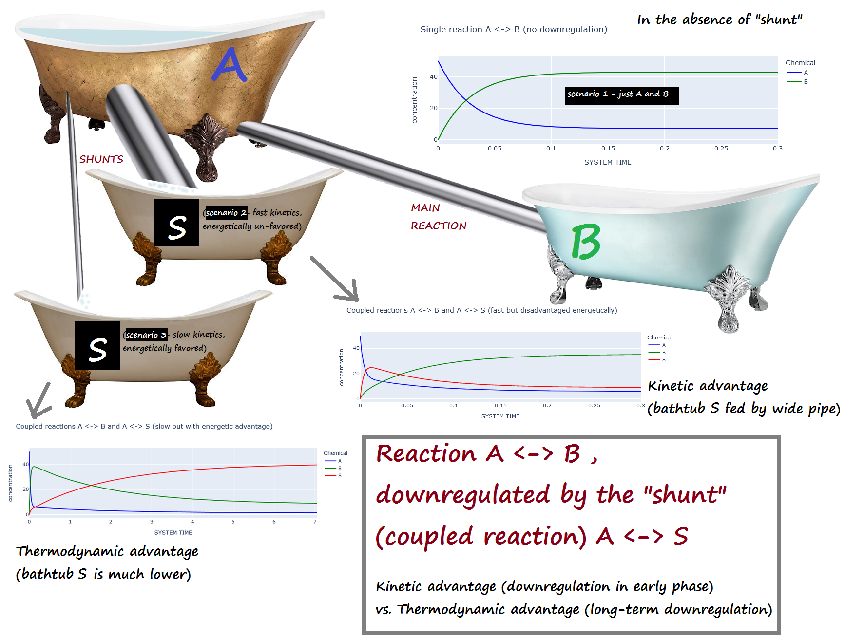
`A <-> B` , downregulated by the "shunt" (coupled reaction) `A <-> S`¶

Kinetic advantage (downregulation in early phase) vs. Thermodynamic advantage (long-term downregulation)¶

Scenario 1 : No downregulation on A <-> B

Scenario 2 : The shunt (A <-> S) has a kinetic advantage but thermodynamic DIS-advantage compared to A <-> B
(i.e. A <-> S is fast, but energetically unfavored)

Scenario 3 : The shunt (A <-> S) is has a kinetic DIS-advantage but a thermodynamic advantage compared to A <-> B
(i.e. A <-> S is slow, but energetically favored)

All reactions 1st order, mostly forward. Taken to equilibrium.

LAST REVISED: May 23, 2023

Bathtub analogy:¶

A is initially full, while B and S are empty.
If the "shunt" S is present, scenario 2 corresponds to a large pipe and a small elevation change...
while scenario 3 corresponds to a narrow pipe and a large elevation change.

Downregulated by shunt

In [1]:

import set_path      # Importing this module will add the project's home directory to sys.path

Added 'D:\Docs\- MY CODE\BioSimulations\life123-Win7' to sys.path

In [2]:

from experiments.get_notebook_info import get_notebook_basename

from src.modules.reactions.reaction_data import ReactionData as chem
from src.modules.reactions.reaction_dynamics import ReactionDynamics

import numpy as np
import plotly.express as px
from src.modules.visualization.graphic_log import GraphicLog

In [3]:

# Initialize the HTML logging (for the graphics)
log_file = get_notebook_basename() + ".log.htm"    # Use the notebook base filename for the log file

# Set up the use of some specified graphic (Vue) components
GraphicLog.config(filename=log_file,
                  components=["vue_cytoscape_1"],
                  extra_js="https://cdnjs.cloudflare.com/ajax/libs/cytoscape/3.21.2/cytoscape.umd.js")

-> Output will be LOGGED into the file 'down_regulate_1.log.htm'

In [ ]:

Scenario 1: A <-> B in the absence of the 2nd reaction ¶

Initialize the System¶

Specify the chemicals and the reaction

In [4]:

# Specify the chemicals
chem_data = chem(names=["A", "B"])

# Reaction A <-> B
chem_data.add_reaction(reactants=["A"], products=["B"],
                       forward_rate=30., reverse_rate=5.)

chem_data.describe_reactions()

Number of reactions: 1 (at temp. 25 C)
0: A <-> B  (kF = 30 / kR = 5 / Delta_G = -4,441.69 / K = 6) | 1st order in all reactants & products

Set the initial concentrations of all the chemicals, in their index order¶

In [5]:

dynamics = ReactionDynamics(reaction_data=chem_data)
dynamics.set_conc([50., 0.], snapshot=True)
dynamics.describe_state()

SYSTEM STATE at Time t = 0:
2 species:
  Species 0 (A). Conc: 50.0
  Species 1 (B). Conc: 0.0

Run the reaction¶

In [6]:

dynamics.set_diagnostics()          # To save diagnostic information about the call to single_compartment_react()

# All of these settings are currently close to the default values... but subject to change; set for repeatability
dynamics.set_thresholds(norm="norm_A", low=0.5, high=1.0, abort=1.44)
dynamics.set_thresholds(norm="norm_B", low=0.08, high=0.5, abort=1.5)
dynamics.set_step_factors(upshift=1.5, downshift=0.5, abort=0.5)
dynamics.set_error_step_factor(0.5)

# The changes of concentrations vary very rapidly early on; automated variable timesteps will take care of that
dynamics.single_compartment_react(initial_step=0.001, reaction_duration=0.3,
                                  snapshots={"initial_caption": "1st reaction step",
                                             "final_caption": "last reaction step"},
                                  variable_steps=True, explain_variable_steps=False)

49 total step(s) taken

In [7]:

dynamics.get_history()

Out[7]:

	SYSTEM TIME	A	B	caption
0	0.000000	50.000000	0.000000	Initial state
1	0.001000	48.500000	1.500000	1st reaction step
2	0.001500	47.776250	2.223750
3	0.002000	47.065166	2.934834
4	0.002500	46.366525	3.633475
5	0.003000	45.680111	4.319889
6	0.003500	45.005709	4.994291
7	0.004000	44.343109	5.656891
8	0.004500	43.692105	6.307895
9	0.005000	43.052493	6.947507
10	0.005500	42.424074	7.575926
11	0.006000	41.806653	8.193347
12	0.006500	41.200037	8.799963
13	0.007250	40.306036	9.693964
14	0.008000	39.435502	10.564498
15	0.008750	38.587820	11.412180
16	0.009500	37.762390	12.237610
17	0.010625	36.556746	13.443254
18	0.011750	35.398574	14.601426
19	0.012875	34.286005	15.713995
20	0.014000	33.217244	16.782756
21	0.015125	32.190565	17.809435
22	0.016250	31.204311	18.795689
23	0.017938	29.783182	20.216818
24	0.018781	29.114585	20.885415
25	0.020047	28.141306	21.858694
26	0.021945	26.746057	23.253943
27	0.023844	25.443516	24.556484
28	0.025742	24.227523	25.772477
29	0.027641	23.092327	26.907673
30	0.029539	22.032560	27.967440
31	0.031438	21.043209	28.956791
32	0.034285	19.657789	30.342211
33	0.037133	18.410451	31.589549
34	0.039980	17.287433	32.712567
35	0.042828	16.276344	33.723656
36	0.045676	15.366028	34.633972
37	0.049947	14.136648	35.863352
38	0.054219	13.091062	36.908938
39	0.058490	12.201794	37.798206
40	0.064897	11.067313	38.932687
41	0.071305	10.187242	39.812758
42	0.080916	9.163174	40.836826
43	0.090526	8.483581	41.516419
44	0.104943	7.807093	42.192907
45	0.126567	7.304364	42.695636
46	0.159004	7.121008	42.878992
47	0.207658	7.158215	42.841785
48	0.280641	7.118985	42.881015
49	0.390114	7.210452	42.789548	last reaction step

In [8]:

dynamics.explain_time_advance()

From time 0 to 0.001, in 1 step of 0.001
From time 0.001 to 0.0065, in 11 steps of 0.0005
From time 0.0065 to 0.0095, in 4 steps of 0.00075
From time 0.0095 to 0.01625, in 6 steps of 0.00113
From time 0.01625 to 0.01794, in 1 step of 0.00169
From time 0.01794 to 0.01878, in 1 step of 0.000844
From time 0.01878 to 0.02005, in 1 step of 0.00127
From time 0.02005 to 0.03144, in 6 steps of 0.0019
From time 0.03144 to 0.04568, in 5 steps of 0.00285
From time 0.04568 to 0.05849, in 3 steps of 0.00427
From time 0.05849 to 0.0713, in 2 steps of 0.00641
From time 0.0713 to 0.09053, in 2 steps of 0.00961
From time 0.09053 to 0.1049, in 1 step of 0.0144
From time 0.1049 to 0.1266, in 1 step of 0.0216
From time 0.1266 to 0.159, in 1 step of 0.0324
From time 0.159 to 0.2077, in 1 step of 0.0487
From time 0.2077 to 0.2806, in 1 step of 0.073
From time 0.2806 to 0.3901, in 1 step of 0.109
(49 steps total)

In [9]:

dynamics.plot_curves(colors=["blue", "green"], title="Single reaction A <-> B (no downregulation)", 
                     show_intervals=True)

Notice the intersection at the exact midpoint of the 2 initial concentrations (50 and 0):¶

In [10]:

dynamics.curve_intersection('A', 'B', t_start=0, t_end=0.1)

Min abs distance found at data row: 27

Out[10]:

(0.02453617850732098, 25.000000000000007)

In [11]:

# Verify that all the reactions have reached equilibrium
dynamics.is_in_equilibrium(tolerance=2)

A <-> B
Final concentrations:  [B] = 42.79 ; [A] = 7.21
1. Ratio of reactant/product concentrations, adjusted for reaction orders: 5.93438
    Formula used:  [B] / [A]
2. Ratio of forward/reverse reaction rates: 6.0
Discrepancy between the two values: 1.094 %
Reaction IS in equilibrium (within 2% tolerance)

Out[11]:

True

In [ ]:

Scenario 2:¶

downregulated by shunt:¶

kinetically fast,¶

but with thermodynamical dis-advantage (i.e. energetically un-favored)¶

In [12]:

# Register the new chemical ("S")
chem_data.add_chemical("S")

# Add the reaction A <-> S (fast shunt, poor thermodynical energetic advantage)
chem_data.add_reaction(reactants=["A"], products=["S"],
                       forward_rate=150., reverse_rate=100.) 

chem_data.describe_reactions()

Number of reactions: 2 (at temp. 25 C)
0: A <-> B  (kF = 30 / kR = 5 / Delta_G = -4,441.69 / K = 6) | 1st order in all reactants & products
1: A <-> S  (kF = 150 / kR = 100 / Delta_G = -1,005.13 / K = 1.5) | 1st order in all reactants & products

In [13]:

# Send a plot of the network of reactions to the HTML log file
graph_data = chem_data.prepare_graph_network()
GraphicLog.export_plot(graph_data, "vue_cytoscape_1")

[GRAPHIC ELEMENT SENT TO LOG FILE `down_regulate_1.log.htm`]

Set the initial concentrations of all the chemicals, in their index order¶

In [14]:

dynamics = ReactionDynamics(reaction_data=chem_data)   # Notice we're over-writing the earlier "dynamics" object
dynamics.set_conc([50., 0, 0.], snapshot=True)
dynamics.describe_state()

SYSTEM STATE at Time t = 0:
3 species:
  Species 0 (A). Conc: 50.0
  Species 1 (B). Conc: 0.0
  Species 2 (S). Conc: 0.0

Run the reaction¶

In [15]:

dynamics.set_diagnostics()         # To save diagnostic information about the call to single_compartment_react()

# All of these settings are currently close to the default values... but subject to change; set for repeatability
dynamics.set_thresholds(norm="norm_A", low=0.5, high=1.0, abort=1.44)
dynamics.set_thresholds(norm="norm_B", low=0.05, high=0.5, abort=1.5)
dynamics.set_step_factors(upshift=1.4, downshift=0.5, abort=0.5)
dynamics.set_error_step_factor(0.333)

# The changes of concentrations vary very rapidly early on; automated variable timesteps will take care of that
dynamics.single_compartment_react(initial_step=0.001, reaction_duration=0.3,
                                  snapshots={"initial_caption": "1st reaction step",
                                             "final_caption": "last reaction step"},
                                  variable_steps=True, explain_variable_steps=False)

INFO: the tentative time step (0.001) leads to a least one norm value > its ABORT threshold:
      -> will backtrack, and re-do step with a SMALLER delta time, multiplied by 0.5 (set to 0.0005) [Step started at t=0, and will rewind there]
INFO: the tentative time step (0.0005) leads to a least one norm value > its ABORT threshold:
      -> will backtrack, and re-do step with a SMALLER delta time, multiplied by 0.5 (set to 0.00025) [Step started at t=0, and will rewind there]
69 total step(s) taken

In [16]:

dynamics.plot_curves(colors=["blue", "green", "red"], 
                     title="Coupled reactions A <-> B and A <-> S (fast but disadvantaged energetically)",
                     show_intervals=True)

Notice how the "alternate (shunt) path" of the reaction, i.e. S (red)¶

has a FAST START (fast kinetics),¶

but EVENTUALLY PETERS OUT (energy dis-advantage)¶

In [17]:

dynamics.explain_time_advance()

From time 0 to 0.0005, in 2 steps of 0.00025
From time 0.0005 to 0.00225, in 14 steps of 0.000125
From time 0.00225 to 0.00295, in 4 steps of 0.000175
From time 0.00295 to 0.00393, in 4 steps of 0.000245
From time 0.00393 to 0.005302, in 4 steps of 0.000343
From time 0.005302 to 0.006743, in 3 steps of 0.00048
From time 0.006743 to 0.009432, in 4 steps of 0.000672
From time 0.009432 to 0.01226, in 3 steps of 0.000941
From time 0.01226 to 0.01753, in 4 steps of 0.00132
From time 0.01753 to 0.0249, in 4 steps of 0.00184
From time 0.0249 to 0.03524, in 4 steps of 0.00258
From time 0.03524 to 0.04608, in 3 steps of 0.00362
From time 0.04608 to 0.06127, in 3 steps of 0.00506
From time 0.06127 to 0.07544, in 2 steps of 0.00709
From time 0.07544 to 0.1151, in 4 steps of 0.00992
From time 0.1151 to 0.1429, in 2 steps of 0.0139
From time 0.1429 to 0.1818, in 2 steps of 0.0194
From time 0.1818 to 0.209, in 1 step of 0.0272
From time 0.209 to 0.2471, in 1 step of 0.0381
From time 0.2471 to 0.3005, in 1 step of 0.0534
(69 steps total)

In [18]:

dynamics.get_history()

Out[18]:

	SYSTEM TIME	A	B	S	caption
0	0.000000	50.000000	0.000000	0.000000	Initial state
1	0.000250	47.750000	0.375000	1.875000	1st reaction step
2	0.000500	45.648594	0.732656	3.618750
3	0.000625	44.667193	0.903381	4.429427
4	0.000750	43.718113	1.070318	5.211569
...	...	...	...	...	...
65	0.162354	6.593940	33.315058	10.091002
66	0.181800	6.375490	33.922608	9.701902
67	0.209024	6.163548	34.512062	9.324390
68	0.247138	5.994349	34.982624	9.023027
69	0.300498	5.900061	35.245013	8.854926	last reaction step

70 rows × 5 columns

In [19]:

# Verify that all the reactions have reached equilibrium
dynamics.is_in_equilibrium()

A <-> B
Final concentrations:  [B] = 35.25 ; [A] = 5.9
1. Ratio of reactant/product concentrations, adjusted for reaction orders: 5.97367
    Formula used:  [B] / [A]
2. Ratio of forward/reverse reaction rates: 6.0
Discrepancy between the two values: 0.4388 %
Reaction IS in equilibrium (within 1% tolerance)

A <-> S
Final concentrations:  [S] = 8.855 ; [A] = 5.9
1. Ratio of reactant/product concentrations, adjusted for reaction orders: 1.50082
    Formula used:  [S] / [A]
2. Ratio of forward/reverse reaction rates: 1.5
Discrepancy between the two values: 0.05463 %
Reaction IS in equilibrium (within 1% tolerance)

Out[19]:

True

In [ ]:

Scenario 3:¶

downregulated by shunt:¶

kinetically slow,¶

but with thermodynamical advantage (i.e. energetically favored)¶

In [20]:

# Specify the chemicals  (notice that we're starting with new objects)
chem_data = chem(names=["A", "B", "S"])

# Reaction A <-> B (as before)
chem_data.add_reaction(reactants=["A"], products=["B"],
                       forward_rate=30., reverse_rate=5.) 

# Reaction A <-> S (slow shunt, excellent thermodynamical energetic advantage)
chem_data.add_reaction(reactants=["A"], products=["S"],
                       forward_rate=3., reverse_rate=0.1)

chem_data.describe_reactions()

Number of reactions: 2 (at temp. 25 C)
0: A <-> B  (kF = 30 / kR = 5 / Delta_G = -4,441.69 / K = 6) | 1st order in all reactants & products
1: A <-> S  (kF = 3 / kR = 0.1 / Delta_G = -8,431.42 / K = 30) | 1st order in all reactants & products

Set the initial concentrations of all the chemicals, in their index order¶

In [21]:

dynamics = ReactionDynamics(reaction_data=chem_data)
dynamics.set_conc([50., 0, 0.], snapshot=True)
dynamics.describe_state()

SYSTEM STATE at Time t = 0:
3 species:
  Species 0 (A). Conc: 50.0
  Species 1 (B). Conc: 0.0
  Species 2 (S). Conc: 0.0

Run the reaction¶

In [22]:

dynamics.set_diagnostics()       # To save diagnostic information about the call to single_compartment_react()

# These settings can be tweaked to make the time resolution finer or coarser
dynamics.set_thresholds(norm="norm_A", low=2.0, high=5.0, abort=10.0)
dynamics.set_thresholds(norm="norm_B", low=0.008, high=0.5, abort=2.0)    # The "low" value here seems especially critical to fend off instabilities
dynamics.set_step_factors(upshift=1.5, downshift=0.25, abort=0.25)
dynamics.set_error_step_factor(0.2)

# The changes of concentrations vary very rapidly early on; automated variable timesteps will take care of that
dynamics.single_compartment_react(initial_step=0.005, reaction_duration=7.0,
                                   snapshots={"initial_caption": "1st reaction step",
                                             "final_caption": "last reaction step"},
                                   variable_steps=True, explain_variable_steps=False)

INFO: the tentative time step (0.005) leads to a least one norm value > its ABORT threshold:
      -> will backtrack, and re-do step with a SMALLER delta time, multiplied by 0.25 (set to 0.00125) [Step started at t=0, and will rewind there]
454 total step(s) taken

In [23]:

dynamics.plot_curves(colors=["blue", "green", "red"], 
                      title="Coupled reactions A <-> B and A <-> S (slow but with energetic advantage)")

Notice how the "alternate (shunt) path" of the reaction, i.e. S (red)¶

has a SLOW START (slow kinetics),¶

but EVENTUALLY DOMINATES (energy advantage)¶

In [24]:

dynamics.explain_time_advance()

From time 0 to 0.0025, in 2 steps of 0.00125
From time 0.0025 to 0.03281, in 97 steps of 0.000313
From time 0.03281 to 0.05859, in 55 steps of 0.000469
From time 0.05859 to 0.07617, in 25 steps of 0.000703
From time 0.07617 to 0.09199, in 15 steps of 0.00105
From time 0.09199 to 0.1062, in 9 steps of 0.00158
From time 0.1062 to 0.1205, in 6 steps of 0.00237
From time 0.1205 to 0.2237, in 29 steps of 0.00356
From time 0.2237 to 0.3999, in 33 steps of 0.00534
From time 0.3999 to 0.6402, in 30 steps of 0.00801
From time 0.6402 to 0.9525, in 26 steps of 0.012
From time 0.9525 to 1.349, in 22 steps of 0.018
From time 1.349 to 1.998, in 24 steps of 0.027
From time 1.998 to 3.66, in 41 steps of 0.0405
From time 3.66 to 4.876, in 20 steps of 0.0608
From time 4.876 to 5.971, in 12 steps of 0.0912
From time 5.971 to 6.929, in 7 steps of 0.137
From time 6.929 to 7.134, in 1 step of 0.205
(454 steps total)

In [25]:

dynamics.get_history()

Out[25]:

	SYSTEM TIME	A	B	S	caption
0	0.000000	50.000000	0.000000	0.000000	Initial state
1	0.001250	47.937500	1.875000	0.187500	1st reaction step
2	0.002500	45.971820	3.660938	0.367242
3	0.002812	45.503468	4.086203	0.410329
4	0.003125	45.040611	4.506413	0.452976
...	...	...	...	...	...
450	6.518546	1.538995	9.356824	39.104182
451	6.655388	1.526366	9.272764	39.200870
452	6.792230	1.514574	9.194376	39.291050
453	6.929072	1.503631	9.121214	39.375155
454	7.134334	1.487983	9.019168	39.492848	last reaction step

455 rows × 5 columns

Check the final equilibrium¶

In [26]:

# Verify that all the reactions have reached equilibrium
dynamics.is_in_equilibrium(tolerance=12)

A <-> B
Final concentrations:  [B] = 9.019 ; [A] = 1.488
1. Ratio of reactant/product concentrations, adjusted for reaction orders: 6.06134
    Formula used:  [B] / [A]
2. Ratio of forward/reverse reaction rates: 6.0
Discrepancy between the two values: 1.022 %
Reaction IS in equilibrium (within 12% tolerance)

A <-> S
Final concentrations:  [S] = 39.49 ; [A] = 1.488
1. Ratio of reactant/product concentrations, adjusted for reaction orders: 26.5412
    Formula used:  [S] / [A]
2. Ratio of forward/reverse reaction rates: 30.0
Discrepancy between the two values: 11.53 %
Reaction IS in equilibrium (within 12% tolerance)

Out[26]:

True

Please note the much-longer timescale from the earlier plots¶

If we look at early time interval, this is what it looks like:

In [27]:

fig = px.line(data_frame=dynamics.get_history().loc[:250], x="SYSTEM TIME", y=["A", "B", "S"], 
              title="Same plot as above, both only showing initial detail",
              color_discrete_sequence = ["blue", "green", "red"],
              labels={"value":"concentration", "variable":"Chemical"})
fig.show()

In [28]:

# Look at where the curves intersect
dynamics.curve_intersection("A", "B", t_start=0, t_end=0.1)

Min abs distance found at data row: 71

Out[28]:

(0.02405919499545674, 23.73396682504195)

In [29]:

dynamics.curve_intersection("A", "S", t_start=0.1, t_end=0.2)

Min abs distance found at data row: 216

Out[29]:

(0.14412951669101942, 6.026379520544665)

In [ ]:

A <-> B , downregulated by the "shunt" (coupled reaction) A <-> S¶

Kinetic advantage (downregulation in early phase) vs. Thermodynamic advantage (long-term downregulation)¶

Bathtub analogy:¶

Scenario 1: A <-> B in the absence of the 2nd reaction¶

Initialize the System¶

Set the initial concentrations of all the chemicals, in their index order¶

Run the reaction¶

Notice the intersection at the exact midpoint of the 2 initial concentrations (50 and 0):¶

Scenario 2:¶

downregulated by shunt:¶

kinetically fast,¶

but with thermodynamical dis-advantage (i.e. energetically un-favored)¶

Set the initial concentrations of all the chemicals, in their index order¶

Run the reaction¶

Notice how the "alternate (shunt) path" of the reaction, i.e. S (red)¶

has a FAST START (fast kinetics),¶

but EVENTUALLY PETERS OUT (energy dis-advantage)¶

Scenario 3:¶

downregulated by shunt:¶

kinetically slow,¶

but with thermodynamical advantage (i.e. energetically favored)¶

Set the initial concentrations of all the chemicals, in their index order¶

Run the reaction¶

Notice how the "alternate (shunt) path" of the reaction, i.e. S (red)¶

has a SLOW START (slow kinetics),¶

but EVENTUALLY DOMINATES (energy advantage)¶

Check the final equilibrium¶

Please note the much-longer timescale from the earlier plots¶

`A <-> B` , downregulated by the "shunt" (coupled reaction) `A <-> S`¶

Scenario 1: A <-> B in the absence of the 2nd reaction ¶