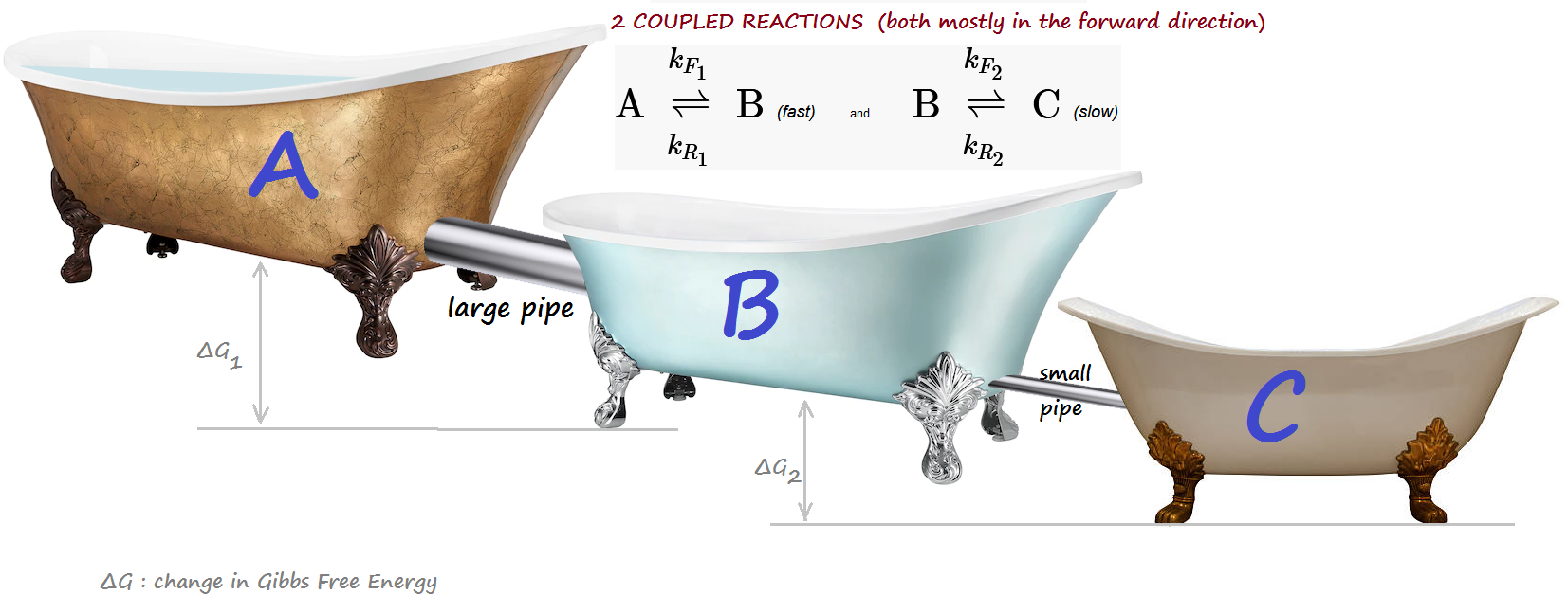
2 COUPLED reactions of different speeds, forming a "cascade":¶

`A <-> B` (fast) and `B <-> C` (slow)¶

All 1st order. Taken to equilibrium. Both reactions are mostly forward. The concentration of the intermediate product B manifests 1 oscillation (transient "overshoot")

(Adaptive variable time resolution is used, with extensive diagnostics.)

LAST REVISED: May 23, 2023

Bathtub analogy:¶

A is initially full, while B and C are empty.
Tubs are progressively lower (reactions are mostly forward.)
A BIG pipe connects A and B: fast kinetics. A small pipe connects B and C: slow kinetics.

INTUITION: B, unable to quickly drain into C while at the same time being blasted by a hefty inflow from A,
will experience a transient surge, in excess of its final equilibrium level.

Compare with the final reaction plot (the red line is B)

2 Coupled Reactions

In [1]:

import set_path      # Importing this module will add the project's home directory to sys.path

Added 'D:\Docs\- MY CODE\BioSimulations\life123-Win7' to sys.path

In [2]:

from experiments.get_notebook_info import get_notebook_basename

from src.modules.reactions.reaction_data import ReactionData as chem
from src.modules.reactions.reaction_dynamics import ReactionDynamics

import numpy as np
import plotly.express as px
from src.modules.visualization.graphic_log import GraphicLog

In [3]:

# Initialize the HTML logging (for the graphics)
log_file = get_notebook_basename() + ".log.htm"    # Use the notebook base filename for the log file

# Set up the use of some specified graphic (Vue) components
GraphicLog.config(filename=log_file,
                  components=["vue_cytoscape_1"],
                  extra_js="https://cdnjs.cloudflare.com/ajax/libs/cytoscape/3.21.2/cytoscape.umd.js")

-> Output will be LOGGED into the file 'cascade_1.log.htm'

Initialize the System¶

Specify the chemicals and the reactions

In [4]:

# Specify the chemicals
chem_data = chem(names=["A", "B", "C"])

# Reaction A <-> B (fast)
chem_data.add_reaction(reactants=["A"], products=["B"],
                       forward_rate=64., reverse_rate=8.) 

# Reaction B <-> C (slow)
chem_data.add_reaction(reactants=["B"], products=["C"],
                       forward_rate=12., reverse_rate=2.) 

print("Number of reactions: ", chem_data.number_of_reactions())

Number of reactions:  2

In [5]:

chem_data.describe_reactions()

Number of reactions: 2 (at temp. 25 C)
0: A <-> B  (kF = 64 / kR = 8 / Delta_G = -5,154.85 / K = 8) | 1st order in all reactants & products
1: B <-> C  (kF = 12 / kR = 2 / Delta_G = -4,441.69 / K = 6) | 1st order in all reactants & products

In [6]:

# Send a plot of the network of reactions to the HTML log file
graph_data = chem_data.prepare_graph_network()
GraphicLog.export_plot(graph_data, "vue_cytoscape_1")

[GRAPHIC ELEMENT SENT TO LOG FILE `cascade_1.log.htm`]

Start the simulation¶

In [7]:

dynamics = ReactionDynamics(reaction_data=chem_data)

Set the initial concentrations of all the chemicals, in their index order¶

In [8]:

dynamics.set_conc([50., 0, 0.], snapshot=True)

In [9]:

dynamics.describe_state()

SYSTEM STATE at Time t = 0:
3 species:
  Species 0 (A). Conc: 50.0
  Species 1 (B). Conc: 0.0
  Species 2 (C). Conc: 0.0

In [10]:

dynamics.get_history()

Out[10]:

	SYSTEM TIME	A	B	C	caption
0	0.0	50.0	0.0	0.0	Initial state

Run the reaction¶

In [11]:

dynamics.set_diagnostics()         # To save diagnostic information about the call to single_compartment_react()

# These settings can be tweaked to make the time resolution finer or coarser
dynamics.set_thresholds(norm="norm_A", low=0.5, high=1.0, abort=1.44)
dynamics.set_thresholds(norm="norm_B", low=0.2, high=0.5, abort=1.5)
dynamics.set_step_factors(upshift=1.4, downshift=0.5, abort=0.5)
dynamics.set_error_step_factor(0.333)

dynamics.single_compartment_react(initial_step=0.02, reaction_duration=0.4,
                                  snapshots={"initial_caption": "1st reaction step",
                                             "final_caption": "last reaction step"},
                                  variable_steps=True, explain_variable_steps=False)

*** CAUTION: negative concentration in chemical `A` in step starting at t=0.  It will be AUTOMATICALLY CORRECTED with a reduction in time step size, as follows:
    INFO: the tentative time step (0.02) leads to a NEGATIVE concentration of `A` from reaction A <-> B (rxn # 0): 
      Baseline value: 50 ; delta conc: -64
      -> will backtrack, and re-do step with a SMALLER delta time, multiplied by 0.333 (set to 0.00666) [Step started at t=0, and will rewind there]
INFO: the tentative time step (0.00666) leads to a least one norm value > its ABORT threshold:
      -> will backtrack, and re-do step with a SMALLER delta time, multiplied by 0.5 (set to 0.00333) [Step started at t=0, and will rewind there]
INFO: the tentative time step (0.00333) leads to a least one norm value > its ABORT threshold:
      -> will backtrack, and re-do step with a SMALLER delta time, multiplied by 0.5 (set to 0.001665) [Step started at t=0, and will rewind there]
INFO: the tentative time step (0.001665) leads to a least one norm value > its ABORT threshold:
      -> will backtrack, and re-do step with a SMALLER delta time, multiplied by 0.5 (set to 0.0008325) [Step started at t=0, and will rewind there]
INFO: the tentative time step (0.0008325) leads to a least one norm value > its ABORT threshold:
      -> will backtrack, and re-do step with a SMALLER delta time, multiplied by 0.5 (set to 0.00041625) [Step started at t=0, and will rewind there]
Some steps were backtracked and re-done, to prevent negative concentrations or excessively large concentration changes
56 total step(s) taken

Plots of changes of concentration with time ¶

In [12]:

dynamics.plot_curves(title="Coupled reactions A <-> B and B <-> C",
                     colors=['blue', 'red', 'green'])

In [13]:

dynamics.curve_intersection("A", "B", t_start=0, t_end=0.05)

Min abs distance found at data row: 26

Out[13]:

(0.011856795047959055, 24.04728216157861)

In [14]:

dynamics.curve_intersection("A", "C", t_start=0, t_end=0.05)

Min abs distance found at data row: 35

Out[14]:

(0.03191446684059964, 8.846824660878902)

In [15]:

dynamics.curve_intersection("B", "C", t_start=0.05, t_end=0.1)

Min abs distance found at data row: 43

Out[15]:

(0.07775497645748508, 23.275670893111585)

In [16]:

dynamics.get_history()

Out[16]:

	SYSTEM TIME	A	B	C	caption
0	0.000000	50.000000	0.000000	0.000000	Initial state
1	0.000416	48.668000	1.332000	0.000000	1st reaction step
2	0.000999	46.859088	3.131597	0.009315
3	0.001290	45.992560	3.987182	0.020259
4	0.001436	45.568372	4.404404	0.027224
5	0.001582	45.148626	4.816459	0.034916
6	0.001727	44.733274	5.223401	0.043326
7	0.001873	44.322268	5.625287	0.052445
8	0.002019	43.915564	6.022172	0.062264
9	0.002223	43.352134	6.570888	0.076978
10	0.002427	42.796954	7.110016	0.093029
11	0.002631	42.249901	7.639705	0.110394
12	0.002916	41.495235	8.368257	0.136509
13	0.003202	40.756024	9.078871	0.165105
14	0.003487	40.031946	9.771934	0.196120
15	0.003887	39.038978	10.718181	0.242841
16	0.004287	38.074442	11.631494	0.294064
17	0.004687	37.137504	12.512868	0.349628
18	0.005246	35.863298	13.703428	0.433274
19	0.005806	34.640063	14.835115	0.524822
20	0.006366	33.465710	15.910421	0.623868
21	0.007149	31.887247	17.340264	0.772489
22	0.007933	30.396901	18.668779	0.934320
23	0.008716	28.989619	19.901992	1.108389
24	0.009813	27.129045	21.503018	1.367938
25	0.010910	25.413143	22.938865	1.647992
26	0.012007	23.830307	24.223361	1.946332
27	0.013543	21.785691	25.827544	2.386764
28	0.015079	19.961745	27.182848	2.855407
29	0.016614	18.333721	28.318692	3.347587
30	0.018764	16.298044	29.638128	4.063828
31	0.020914	14.565177	30.623792	4.811031
32	0.023065	13.087710	31.331838	5.580452
33	0.026075	11.320931	32.000484	6.678584
34	0.029085	9.910612	32.295130	7.794258
35	0.033299	8.326464	32.311839	9.361697
36	0.037513	7.170125	31.913104	10.916771
37	0.043412	5.969043	30.983661	13.047296
38	0.049312	5.177600	29.735519	15.086881
39	0.055212	4.626082	28.359882	17.014036
40	0.061112	4.217880	26.961059	18.821061
41	0.067011	3.897786	25.594481	20.507733
42	0.072911	3.634055	24.288192	22.077754
43	0.081171	3.317927	22.561698	24.120374
44	0.089430	3.054828	20.987041	25.958131
45	0.097690	2.826759	19.563784	27.609457
46	0.105949	2.625206	18.282356	29.092438
47	0.117513	2.373651	16.669846	30.956503
48	0.129076	2.159093	15.287204	32.553704
49	0.140640	1.975416	14.102475	33.922109
50	0.156829	1.755138	12.681443	35.563419
51	0.173017	1.579048	11.545423	36.875529
52	0.195682	1.381966	10.273992	38.344042
53	0.227412	1.183530	8.993814	39.822657
54	0.271834	1.014931	7.906136	41.078933
55	0.334025	0.908803	7.221459	41.869738
56	0.421092	0.874697	7.001500	42.123803	last reaction step

In [17]:

dynamics.explain_time_advance()

From time 0 to 0.0004163, in 1 step of 0.000416
From time 0.0004163 to 0.000999, in 1 step of 0.000583
From time 0.000999 to 0.00129, in 1 step of 0.000291
From time 0.00129 to 0.002019, in 5 steps of 0.000146
From time 0.002019 to 0.002631, in 3 steps of 0.000204
From time 0.002631 to 0.003487, in 3 steps of 0.000286
From time 0.003487 to 0.004687, in 3 steps of 0.0004
From time 0.004687 to 0.006366, in 3 steps of 0.00056
From time 0.006366 to 0.008716, in 3 steps of 0.000784
From time 0.008716 to 0.01201, in 3 steps of 0.0011
From time 0.01201 to 0.01661, in 3 steps of 0.00154
From time 0.01661 to 0.02306, in 3 steps of 0.00215
From time 0.02306 to 0.02908, in 2 steps of 0.00301
From time 0.02908 to 0.03751, in 2 steps of 0.00421
From time 0.03751 to 0.07291, in 6 steps of 0.0059
From time 0.07291 to 0.1059, in 4 steps of 0.00826
From time 0.1059 to 0.1406, in 3 steps of 0.0116
From time 0.1406 to 0.173, in 2 steps of 0.0162
From time 0.173 to 0.1957, in 1 step of 0.0227
From time 0.1957 to 0.2274, in 1 step of 0.0317
From time 0.2274 to 0.2718, in 1 step of 0.0444
From time 0.2718 to 0.334, in 1 step of 0.0622
From time 0.334 to 0.4211, in 1 step of 0.0871
(56 steps total)

Check the final equilibrium¶

In [18]:

# Verify that all the reactions have reached equilibrium
dynamics.is_in_equilibrium()

A <-> B
Final concentrations:  [B] = 7.001 ; [A] = 0.8747
1. Ratio of reactant/product concentrations, adjusted for reaction orders: 8.00449
    Formula used:  [B] / [A]
2. Ratio of forward/reverse reaction rates: 8.0
Discrepancy between the two values: 0.05606 %
Reaction IS in equilibrium (within 1% tolerance)

B <-> C
Final concentrations:  [C] = 42.12 ; [B] = 7.001
1. Ratio of reactant/product concentrations, adjusted for reaction orders: 6.0164
    Formula used:  [C] / [B]
2. Ratio of forward/reverse reaction rates: 6.0
Discrepancy between the two values: 0.2733 %
Reaction IS in equilibrium (within 1% tolerance)

Out[18]:

True

In [ ]:

EVERYTHING BELOW IS FOR DIAGNOSTIC INSIGHT¶

Perform some verification¶

Take a peek at the diagnostic data saved during the earlier reaction simulation¶

In [19]:

# Concentration increments due to reaction 0 (A <-> B)
# Note that [C] is not affected
dynamics.get_diagnostic_rxn_data(rxn_index=0)

Reaction:  A <-> B

Out[19]:

	START_TIME	Delta A	Delta B	Delta C	time_step	caption
0	0.000000	NaN	NaN	NaN	0.020000	aborted: neg. conc. in `A`
1	0.000000	-21.312000	21.312000	0.0	0.006660	aborted: excessive norm value(s)
2	0.000000	-10.656000	10.656000	0.0	0.003330	aborted: excessive norm value(s)
3	0.000000	-5.328000	5.328000	0.0	0.001665	aborted: excessive norm value(s)
4	0.000000	-2.664000	2.664000	0.0	0.000833	aborted: excessive norm value(s)
...	...	...	...	...	...	...
56	0.173017	-0.197082	0.197082	0.0	0.022664
57	0.195682	-0.198437	0.198437	0.0	0.031730
58	0.227412	-0.168599	0.168599	0.0	0.044422
59	0.271834	-0.106128	0.106128	0.0	0.062191
60	0.334025	-0.034106	0.034106	0.0	0.087067

61 rows × 6 columns

In [20]:

# Concentration increments due to reaction 1 (B <-> C)
# Note that [A] is not affected.  
# Also notice that the 0-th row from the A <-> B reaction isn't seen here, because that step was aborted
# early on, before even getting to THIS reaction
dynamics.get_diagnostic_rxn_data(rxn_index=1)

Reaction:  B <-> C

Out[20]:

	START_TIME	Delta B	Delta C	time_step	caption
0	0.000000	0.000000	0.000000	0.006660	aborted: excessive norm value(s)
1	0.000000	0.000000	0.000000	0.003330	aborted: excessive norm value(s)
2	0.000000	0.000000	0.000000	0.001665	aborted: excessive norm value(s)
3	0.000000	0.000000	0.000000	0.000833	aborted: excessive norm value(s)
4	0.000000	0.000000	0.000000	0.000416
5	0.000416	-0.009315	0.009315	0.000583
6	0.000999	-0.010944	0.010944	0.000291
7	0.001290	-0.006965	0.006965	0.000146
8	0.001436	-0.007692	0.007692	0.000146
9	0.001582	-0.008410	0.008410	0.000146
10	0.001727	-0.009119	0.009119	0.000146
11	0.001873	-0.009819	0.009819	0.000146
12	0.002019	-0.014714	0.014714	0.000204
13	0.002223	-0.016051	0.016051	0.000204
14	0.002427	-0.017364	0.017364	0.000204
15	0.002631	-0.026115	0.026115	0.000286
16	0.002916	-0.028596	0.028596	0.000286
17	0.003202	-0.031015	0.031015	0.000286
18	0.003487	-0.046721	0.046721	0.000400
19	0.003887	-0.051223	0.051223	0.000400
20	0.004287	-0.055563	0.055563	0.000400
21	0.004687	-0.083646	0.083646	0.000560
22	0.005246	-0.091548	0.091548	0.000560
23	0.005806	-0.099046	0.099046	0.000560
24	0.006366	-0.148620	0.148620	0.000784
25	0.007149	-0.161831	0.161831	0.000784
26	0.007933	-0.174069	0.174069	0.000784
27	0.008716	-0.259548	0.259548	0.001097
28	0.009813	-0.280054	0.280054	0.001097
29	0.010910	-0.298340	0.298340	0.001097
30	0.012007	-0.440432	0.440432	0.001536
31	0.013543	-0.468643	0.468643	0.001536
32	0.015079	-0.492180	0.492180	0.001536
33	0.016614	-0.716241	0.716241	0.002150
34	0.018764	-0.747203	0.747203	0.002150
35	0.020914	-0.769421	0.769421	0.002150
36	0.023065	-1.098132	1.098132	0.003010
37	0.026075	-1.115673	1.115673	0.003010
38	0.029085	-1.567439	1.567439	0.004214
39	0.033299	-1.555074	1.555074	0.004214
40	0.037513	-2.130525	2.130525	0.005900
41	0.043412	-2.039585	2.039585	0.005900
42	0.049312	-1.927155	1.927155	0.005900
43	0.055212	-1.807025	1.807025	0.005900
44	0.061112	-1.686672	1.686672	0.005900
45	0.067011	-1.570021	1.570021	0.005900
46	0.072911	-2.042621	2.042621	0.008260
47	0.081171	-1.837757	1.837757	0.008260
48	0.089430	-1.651326	1.651326	0.008260
49	0.097690	-1.482981	1.482981	0.008260
50	0.105949	-1.864064	1.864064	0.011563
51	0.117513	-1.597201	1.597201	0.011563
52	0.129076	-1.368405	1.368405	0.011563
53	0.140640	-1.641310	1.641310	0.016189
54	0.156829	-1.312110	1.312110	0.016189
55	0.173017	-1.468513	1.468513	0.022664
56	0.195682	-1.478615	1.478615	0.031730
57	0.227412	-1.256276	1.256276	0.044422
58	0.271834	-0.790805	0.790805	0.062191
59	0.334025	-0.254065	0.254065	0.087067

In [ ]:

Provide a detailed explanation of all the steps/substeps of the reactions, from the saved diagnostic data¶

In [ ]:

Re-run with very small constanst steps¶

We'll use constant steps of size 0.0005, which is 1/4 of the smallest steps (the "substep" size) previously used in the variable-step run

In [21]:

dynamics2 = ReactionDynamics(reaction_data=chem_data)

In [22]:

dynamics2.set_conc([50., 0, 0.], snapshot=True)

In [23]:

dynamics2.single_compartment_react(initial_step=0.0005, reaction_duration=0.4,
                                  snapshots={"initial_caption": "1st reaction step",
                                             "final_caption": "last reaction step"},
                                  )      

800 total step(s) taken

In [24]:

fig = px.line(data_frame=dynamics2.get_history(), x="SYSTEM TIME", y=["A", "B", "C"], 
              title="Coupled reactions A <-> B and B <-> C (run with constant steps)",
              color_discrete_sequence = ['blue', 'red', 'green'],
              labels={"value":"concentration", "variable":"Chemical"})
fig.show()

In [25]:

dynamics2.curve_intersection(t_start=0, t_end=0.05, chem1="A", chem2="B")

Min abs distance found at data row: 24

Out[25]:

(0.011934802021672202, 24.03028826511689)

In [26]:

dynamics2.curve_intersection(t_start=0, t_end=0.05, chem1="A", chem2="C")

Min abs distance found at data row: 65

Out[26]:

(0.03259520587890533, 9.081194286771336)

In [27]:

dynamics2.curve_intersection(t_start=0.05, t_end=0.1, chem1="B", chem2="C")

Min abs distance found at data row: 159

Out[27]:

(0.07932921476313338, 23.238745930657448)

In [28]:

df2 = dynamics2.get_history()
df2

Out[28]:

	SYSTEM TIME	A	B	C	caption
0	0.0000	50.000000	0.000000	0.000000	Initial state
1	0.0005	48.400000	1.600000	0.000000	1st reaction step
2	0.0010	46.857600	3.132800	0.009600
3	0.0015	45.370688	4.600925	0.028387
4	0.0020	43.937230	6.006806	0.055964
...	...	...	...	...	...
796	0.3980	0.925494	7.329151	41.745354
797	0.3985	0.925195	7.327221	41.747584
798	0.3990	0.924898	7.325303	41.749800
799	0.3995	0.924602	7.323396	41.752002
800	0.4000	0.924309	7.321501	41.754190	last reaction step

801 rows × 5 columns

Notice that we now did 801 steps - vs. the 56 of the earlier variable-resolution run!¶

Let's compare some entries with the coarser previous variable-time run¶

Let's compare the plots of [B] from the earlier (variable-step) run, and the latest (high-precision, fixed-step) one:¶

In [29]:

# Earlier run (using variable time steps)
fig1 = px.line(data_frame=dynamics.get_history(), x="SYSTEM TIME", y=["B"], 
              color_discrete_sequence = ['red'],
              labels={"value":"concentration", "variable":"Variable-step run"})
fig1.show()

In [30]:

# Latest run (high-precision result from fine fixed-resolution run)
fig2 = px.line(data_frame=dynamics2.get_history(), x="SYSTEM TIME", y=["B"], 
              color_discrete_sequence = ['orange'],
              labels={"value":"concentration", "variable":"Fine fixed-step run"})
fig2.show()

In [31]:

import plotly.graph_objects as go

all_fig = go.Figure(data=fig1.data + fig2.data)    # Note that the + is concatenating lists
all_fig.update_layout(title="The 2 runs contrasted")
all_fig['data'][0]['name']="B (variable steps)"
all_fig['data'][1]['name']="B (fixed high precision)"
all_fig.show()

In [ ]:

2 COUPLED reactions of different speeds, forming a "cascade":¶

A <-> B (fast) and B <-> C (slow)¶

Bathtub analogy:¶

Initialize the System¶

Start the simulation¶

Set the initial concentrations of all the chemicals, in their index order¶

Run the reaction¶

Plots of changes of concentration with time¶

Check the final equilibrium¶

EVERYTHING BELOW IS FOR DIAGNOSTIC INSIGHT¶

Perform some verification¶

Take a peek at the diagnostic data saved during the earlier reaction simulation¶

Provide a detailed explanation of all the steps/substeps of the reactions, from the saved diagnostic data¶

Re-run with very small constanst steps¶

Notice that we now did 801 steps - vs. the 56 of the earlier variable-resolution run!¶

Let's compare some entries with the coarser previous variable-time run¶

Let's compare the plots of [B] from the earlier (variable-step) run, and the latest (high-precision, fixed-step) one:¶

`A <-> B` (fast) and `B <-> C` (slow)¶

Plots of changes of concentration with time ¶