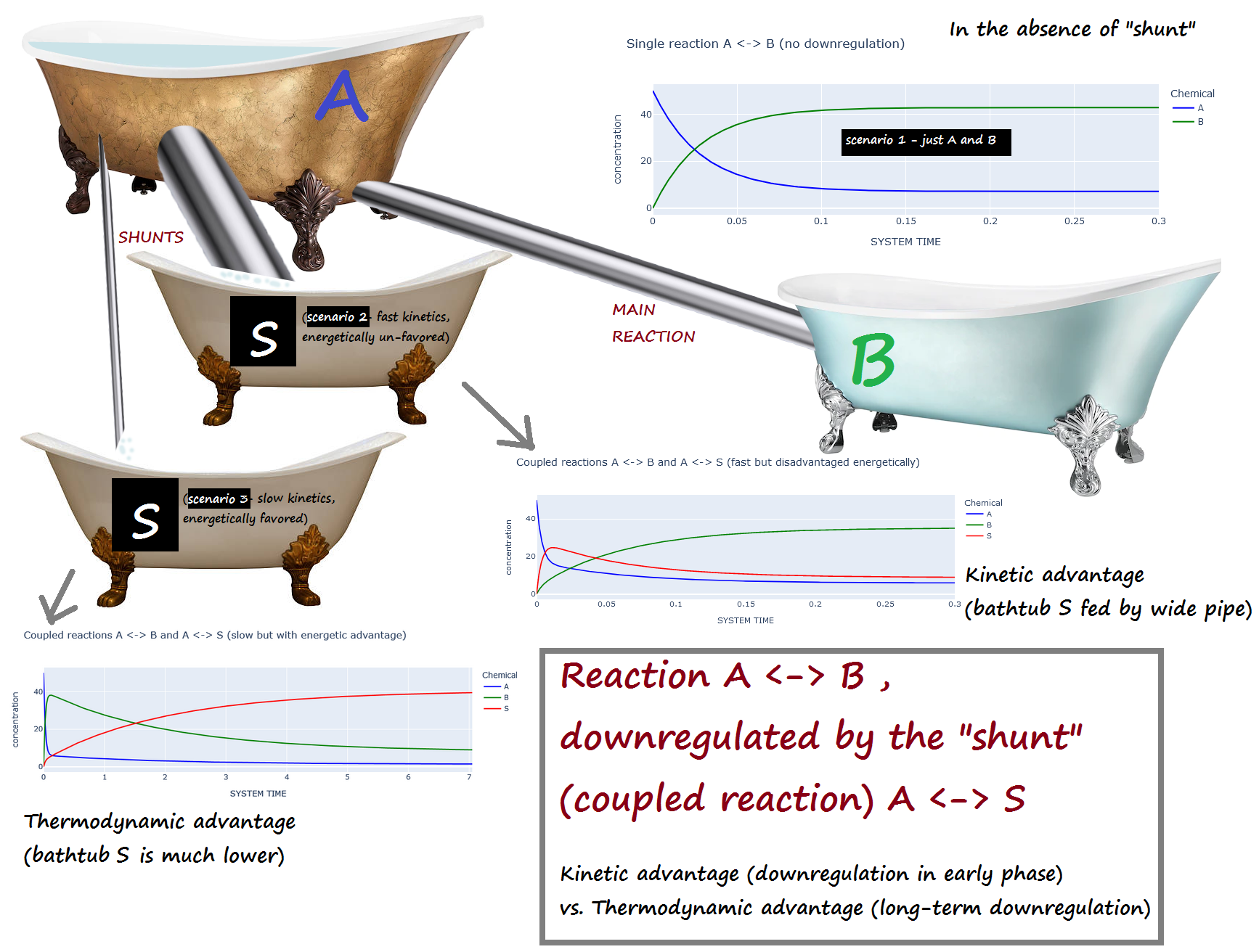
`A <-> B` , downregulated by the "shunt" (coupled reaction) `A <-> S`¶

Kinetic advantage (downregulation in early phase) vs. Thermodynamic advantage (long-term downregulation)¶

Scenario 1 : No downregulation on A <-> B

Scenario 2 : The shunt (A <-> S) has a kinetic advantage but thermodynamic DIS-advantage compared to A <-> B
(i.e. A <-> S is fast, but energetically unfavored)

Scenario 3 : The shunt (A <-> S) is has a kinetic DIS-advantage but a thermodynamic advantage compared to A <-> B
(i.e. A <-> S is slow, but energetically favored)

All reactions 1st order, mostly forward. Taken to equilibrium.

LAST REVISED: Feb. 5, 2023

Bathtub analogy:¶

A is initially full, while B and S are empty.
If the "shunt" S is present, scenario 2 corresponds to a large pipe and a small elevation change...
while scenario 3 corresponds to a narrow pipe and a large elevation change.

Downregulated by shunt

In [1]:

# Extend the sys.path variable, to contain the project's root directory
import set_path
set_path.add_ancestor_dir_to_syspath(2)  # The number of levels to go up 
                                         # to reach the project's home, from the folder containing this notebook

Added 'D:\Docs\- MY CODE\BioSimulations\life123-Win7' to sys.path

In [2]:

from experiments.get_notebook_info import get_notebook_basename

from src.modules.reactions.reaction_data import ReactionData as chem
from src.modules.reactions.reaction_dynamics import ReactionDynamics

import numpy as np
import plotly.express as px
from src.modules.visualization.graphic_log import GraphicLog

In [3]:

# Initialize the HTML logging (for the graphics)
log_file = get_notebook_basename() + ".log.htm"    # Use the notebook base filename for the log file

# Set up the use of some specified graphic (Vue) components
GraphicLog.config(filename=log_file,
                  components=["vue_cytoscape_1"],
                  extra_js="https://cdnjs.cloudflare.com/ajax/libs/cytoscape/3.21.2/cytoscape.umd.js")

-> Output will be LOGGED into the file 'down_regulate_1.log.htm'

Scenario 1: A <-> B in the absence of the 2nd reaction ¶

Initialize the System¶

Specify the chemicals and the reaction

In [4]:

# Specify the chemicals
chem_data = chem(names=["A", "B"])

# Reaction A <-> B
chem_data.add_reaction(reactants=["A"], products=["B"],
                       forward_rate=30., reverse_rate=5.)

chem_data.describe_reactions()

Number of reactions: 1 (at temp. 25 C)
0: A <-> B  (kF = 30 / kR = 5 / Delta_G = -4,441.69 / K = 6) | 1st order in all reactants & products

Set the initial concentrations of all the chemicals, in their index order¶

In [5]:

dynamics = ReactionDynamics(reaction_data=chem_data)
dynamics.set_conc([50., 0.], snapshot=True)
dynamics.describe_state()

SYSTEM STATE at Time t = 0:
2 species:
  Species 0 (A). Conc: 50.0
  Species 1 (B). Conc: 0.0

Run the reaction¶

In [6]:

dynamics.set_diagnostics()          # To save diagnostic information about the call to single_compartment_react()
#dynamics.verbose_list = [1, 2, 3]   # Uncomment for detailed run information (meant for debugging the adaptive variable time step)

# The changes of concentrations vary very rapidly early on; 
# so, we'll be using the dynamic_substeps option to increase time resolution,
# as long as the reaction remains "fast" (based on a threshold of % change, as specified by fast_threshold)
dynamics.single_compartment_react(time_step=0.001, reaction_duration=0.05,
                                  snapshots={"initial_caption": "1st reaction step",
                                             "final_caption": "last reaction step"},
                                  dynamic_substeps=4, rel_fast_threshold=25)

single_compartment_react(): setting abs_fast_threshold to 250.0
50 total step(s) taken

In [7]:

df_iterm = dynamics.get_history()
df_iterm

Out[7]:

	SYSTEM TIME	A	B	caption
0	0.00000	50.000000	0.000000	Initial state
1	0.00025	49.625000	0.375000	Interm. step, due to the fast rxns: [0]
2	0.00050	49.253281	0.746719	Interm. step, due to the fast rxns: [0]
3	0.00075	48.884815	1.115185	Interm. step, due to the fast rxns: [0]
4	0.00100	48.519573	1.480427	1st reaction step
...	...	...	...	...
196	0.04900	14.797598	35.202402
197	0.04925	14.730619	35.269381	Interm. step, due to the fast rxns: [0]
198	0.04950	14.664226	35.335774	Interm. step, due to the fast rxns: [0]
199	0.04975	14.598414	35.401586	Interm. step, due to the fast rxns: [0]
200	0.05000	14.533178	35.466822	last reaction step

201 rows × 4 columns

In [8]:

# Continue running the reaction at lover resolution
dynamics.single_compartment_react(time_step=0.002, reaction_duration=0.25,
                                  snapshots={"initial_caption": "1st reaction step",
                                             "final_caption": "last reaction step"},
                                  dynamic_substeps=4, rel_fast_threshold=10)

single_compartment_react(): setting abs_fast_threshold to 50.0
125 total step(s) taken

In [9]:

df = dynamics.get_history()
df

Out[9]:

	SYSTEM TIME	A	B	caption
0	0.00000	50.000000	0.000000	Initial state
1	0.00025	49.625000	0.375000	Interm. step, due to the fast rxns: [0]
2	0.00050	49.253281	0.746719	Interm. step, due to the fast rxns: [0]
3	0.00075	48.884815	1.115185	Interm. step, due to the fast rxns: [0]
4	0.00100	48.519573	1.480427	1st reaction step
...	...	...	...	...
393	0.29200	7.144047	42.855953
394	0.29400	7.143964	42.856036
395	0.29600	7.143886	42.856114
396	0.29800	7.143814	42.856186
397	0.30000	7.143747	42.856253	last reaction step

398 rows × 4 columns

In [10]:

dynamics.explain_time_advance()

From time 0 to 0.05, in 200 substeps of 0.00025 (each 1/4 of full step)
From time 0.05 to 0.098, in 96 substeps of 0.0005 (each 1/4 of full step)
From time 0.098 to 0.3, in 101 FULL steps of 0.002

In [11]:

# Verify that all the reactions have reached equilibrium
dynamics.is_in_equilibrium()

A <-> B
Final concentrations:  [B] = 42.86 ; [A] = 7.144
1. Ratio of reactant/product concentrations, adjusted for reaction orders: 5.99913
    Formula used:  [B] / [A]
2. Ratio of forward/reverse reaction rates: 6.0
Discrepancy between the two values: 0.01453 %
Reaction IS in equilibrium (within 1% tolerance)

Out[11]:

True

In [12]:

dynamics.plot_curves(colors=["blue", "green"], title="Single reaction A <-> B (no downregulation)")

In [ ]:

Scenario 2:¶

downregulated by shunt:¶

kinetically fast,¶

but with thermodynamical dis-advantage (i.e. energetically un-favored)¶

In [13]:

# Register the new chemical ("S")
chem_data.add_chemical("S")

# Add the reaction A <-> S (fast shunt, poor thermodynical energetic advantage)
chem_data.add_reaction(reactants=["A"], products=["S"],
                       forward_rate=150., reverse_rate=100.) 

chem_data.describe_reactions()

Number of reactions: 2 (at temp. 25 C)
0: A <-> B  (kF = 30 / kR = 5 / Delta_G = -4,441.69 / K = 6) | 1st order in all reactants & products
1: A <-> S  (kF = 150 / kR = 100 / Delta_G = -1,005.13 / K = 1.5) | 1st order in all reactants & products

In [14]:

# Send a plot of the network of reactions to the HTML log file
graph_data = chem_data.prepare_graph_network()
GraphicLog.export_plot(graph_data, "vue_cytoscape_1")

[GRAPHIC ELEMENT SENT TO LOG FILE `down_regulate_1.log.htm`]

Set the initial concentrations of all the chemicals, in their index order¶

In [15]:

dynamics = ReactionDynamics(reaction_data=chem_data)   # Notice we're over-writing the earlier "dynamics" object
dynamics.set_conc([50., 0, 0.], snapshot=True)
dynamics.describe_state()

SYSTEM STATE at Time t = 0:
3 species:
  Species 0 (A). Conc: 50.0
  Species 1 (B). Conc: 0.0
  Species 2 (S). Conc: 0.0

Run the reaction¶

In [16]:

dynamics.set_diagnostics()         # To save diagnostic information about the call to single_compartment_react()
#dynamics.verbose_list = [1, 2, 3]  # Uncomment for detailed run information (meant for debugging the adaptive variable time step)

# The changes of concentrations vary very rapidly early on; 
# so, we'll be using the dynamic_substeps option to increase time resolution,
# as long as the reaction remains "fast" (based on a threshold of % change, as specified by fast_threshold)
dynamics.single_compartment_react(time_step=0.001, reaction_duration=0.05,
                                  snapshots={"initial_caption": "1st reaction step",
                                             "final_caption": "last reaction step"},
                                  dynamic_substeps=4, rel_fast_threshold=10)

single_compartment_react(): setting abs_fast_threshold to 100.0
50 total step(s) taken

In [17]:

# Continue running the reaction at lover resolution
dynamics.single_compartment_react(time_step=0.002, reaction_duration=0.25,
                                  snapshots={"initial_caption": "1st reaction step",
                                             "final_caption": "last reaction step"},
                                  dynamic_substeps=4, rel_fast_threshold=10)

single_compartment_react(): setting abs_fast_threshold to 50.0
125 total step(s) taken

In [18]:

df = dynamics.get_history()
df

Out[18]:

	SYSTEM TIME	A	B	S	caption
0	0.00000	50.000000	0.000000	0.000000	Initial state
1	0.00025	47.750000	0.375000	1.875000	Interm. step, due to the fast rxns: [0, 1]
2	0.00050	45.648594	0.732656	3.618750	Interm. step, due to the fast rxns: [0, 1]
3	0.00075	43.685792	1.074105	5.240104	Interm. step, due to the fast rxns: [0, 1]
4	0.00100	41.852276	1.400406	6.747318	1st reaction step
...	...	...	...	...	...
465	0.29200	5.990345	34.993770	9.015885
466	0.29400	5.986936	35.003253	9.009812
467	0.29600	5.983634	35.012436	9.003930
468	0.29800	5.980436	35.021330	8.998234
469	0.30000	5.977339	35.029943	8.992718	last reaction step

470 rows × 5 columns

Check the final equilibrium¶

In [19]:

# Verify that all the reactions have reached equilibrium
dynamics.is_in_equilibrium(tolerance=3)

A <-> B
Final concentrations:  [B] = 35.03 ; [A] = 5.977
1. Ratio of reactant/product concentrations, adjusted for reaction orders: 5.86046
    Formula used:  [B] / [A]
2. Ratio of forward/reverse reaction rates: 6.0
Discrepancy between the two values: 2.326 %
Reaction IS in equilibrium (within 3% tolerance)

A <-> S
Final concentrations:  [S] = 8.993 ; [A] = 5.977
1. Ratio of reactant/product concentrations, adjusted for reaction orders: 1.50447
    Formula used:  [S] / [A]
2. Ratio of forward/reverse reaction rates: 1.5
Discrepancy between the two values: 0.2979 %
Reaction IS in equilibrium (within 3% tolerance)

Out[19]:

True

Plots of changes of concentration with time ¶

In [20]:

dynamics.plot_curves(colors=["blue", "green", "red"], 
                     title="Coupled reactions A <-> B and A <-> S (fast but disadvantaged energetically)")

Notice how the "alternate (shunt) path" of the reaction, i.e. S (red)¶

has a FAST START (fast kinetics),¶

but EVENTUALLY PETERS OUT (energy dis-advantage)¶

In [21]:

# Verify that the stoichiometry is respected at every reaction step/substep (NOTE: it requires earlier activation of saving diagnostic data)
dynamics.stoichiometry_checker_entire_run()

Out[21]:

True

In [ ]:

Scenario 3:¶

downregulated by shunt:¶

kinetically slow,¶

but with thermodynamical advantage (i.e. energetically favored)¶

In [22]:

# Specify the chemicals  (notice that we're starting with new objects)
chem_data3 = chem(names=["A", "B", "S"])

# Reaction A <-> B (as before)
chem_data3.add_reaction(reactants=["A"], products=["B"],
                       forward_rate=30., reverse_rate=5.) 

# Reaction A <-> S (slow shunt, excellent thermodynamical energetic advantage)
chem_data3.add_reaction(reactants=["A"], products=["S"],
                       forward_rate=3., reverse_rate=0.1)

chem_data3.describe_reactions()

Number of reactions: 2 (at temp. 25 C)
0: A <-> B  (kF = 30 / kR = 5 / Delta_G = -4,441.69 / K = 6) | 1st order in all reactants & products
1: A <-> S  (kF = 3 / kR = 0.1 / Delta_G = -8,431.42 / K = 30) | 1st order in all reactants & products

Set the initial concentrations of all the chemicals, in their index order¶

In [23]:

dynamics3 = ReactionDynamics(reaction_data=chem_data3)
dynamics3.set_conc([50., 0, 0.], snapshot=True)
dynamics3.describe_state()

SYSTEM STATE at Time t = 0:
3 species:
  Species 0 (A). Conc: 50.0
  Species 1 (B). Conc: 0.0
  Species 2 (S). Conc: 0.0

Run the reaction¶

In [24]:

dynamics3.set_diagnostics()       # To save diagnostic information about the call to single_compartment_react()
#dynamics3.verbose_list = [1, 2, 3]  # Uncomment for detailed run information (meant for debugging the adaptive variable time step)

# The changes of concentrations vary very rapidly early on; 
# so, we'll be using the dynamic_substeps option to increase time resolution,
# as long as the reaction remains "fast" (based on a threshold of % change, as specified by fast_threshold)
dynamics3.single_compartment_react(time_step=0.005, reaction_duration=0.3,
                                   snapshots={"initial_caption": "1st reaction step",
                                             "final_caption": "last reaction step"},
                                   dynamic_substeps=5, rel_fast_threshold=10)

single_compartment_react(): setting abs_fast_threshold to 20.0
60 total step(s) taken

In [25]:

# Continue running the reaction at lover resolution
dynamics3.single_compartment_react(time_step=0.25, reaction_duration=6.7,
                                   snapshots={"initial_caption": "1st reaction step",
                                             "final_caption": "last reaction step"},
                                   dynamic_substeps=5, rel_fast_threshold=10)

single_compartment_react(): setting abs_fast_threshold to 0.4
27 total step(s) taken

In [26]:

df3 = dynamics3.get_history()
df3

Out[26]:

	SYSTEM TIME	A	B	S	caption
0	0.000	50.000000	0.000000	0.000000	Initial state
1	0.001	48.350000	1.500000	0.150000	Interm. step, due to the fast rxns: [0, 1]
2	0.002	46.761965	2.943000	0.295035	Interm. step, due to the fast rxns: [0, 1]
3	0.003	45.233565	4.331144	0.435291	Interm. step, due to the fast rxns: [0, 1]
4	0.004	43.762556	5.666495	0.570949	Interm. step, due to the fast rxns: [0, 1]
...	...	...	...	...	...
275	6.850	1.511216	9.171961	39.316824	Interm. step, due to the fast rxns: [0, 1]
276	6.900	1.507284	9.145794	39.346922	Interm. step, due to the fast rxns: [0, 1]
277	6.950	1.503449	9.120272	39.376280	Interm. step, due to the fast rxns: [0, 1]
278	7.000	1.499708	9.095377	39.404916	Interm. step, due to the fast rxns: [0, 1]
279	7.050	1.496059	9.071094	39.432847	last reaction step

280 rows × 5 columns

Check the final equilibrium¶

In [27]:

# Verify that all the reactions have reached equilibrium
dynamics3.is_in_equilibrium(tolerance=13)

A <-> B
Final concentrations:  [B] = 9.071 ; [A] = 1.496
1. Ratio of reactant/product concentrations, adjusted for reaction orders: 6.06333
    Formula used:  [B] / [A]
2. Ratio of forward/reverse reaction rates: 6.0
Discrepancy between the two values: 1.055 %
Reaction IS in equilibrium (within 13% tolerance)

A <-> S
Final concentrations:  [S] = 39.43 ; [A] = 1.496
1. Ratio of reactant/product concentrations, adjusted for reaction orders: 26.3578
    Formula used:  [S] / [A]
2. Ratio of forward/reverse reaction rates: 30.0
Discrepancy between the two values: 12.14 %
Reaction IS in equilibrium (within 13% tolerance)

Out[27]:

True

Plots of changes of concentration with time ¶

In [28]:

dynamics3.plot_curves(colors=["blue", "green", "red"], 
                      title="Coupled reactions A <-> B and A <-> S (slow but with energetic advantage)")

Notice how the "alternate (shunt) path" of the reaction, i.e. S (red)¶

has a SLOW START (slow kinetics),¶

but EVENTUALLY DOMINATES (energy advantage)¶

Please note the much-longer timescale from the earlier plots¶

If we look at the initial [0-0.1] interval, this is what it looks like:

In [29]:

fig = px.line(data_frame=dynamics3.get_history().loc[:96], x="SYSTEM TIME", y=["A", "B", "S"], 
              title="Same as above, both only showing initial detail",
              color_discrete_sequence = ['blue', 'green', 'red'],
              labels={"value":"concentration", "variable":"Chemical"})
fig.show()

In [30]:

dynamics3.curve_intersection(t_start=0, t_end=0.08, var1="A", var2="B")

Min abs distance found at row: 24

Out[30]:

(0.02378914647211626, 23.73644141393734)

In [31]:

# Verify that the stoichiometry is respected at every reaction step/substep (NOTE: it requires earlier activation of saving diagnostic data)
dynamics.stoichiometry_checker_entire_run()

Out[31]:

True

In [ ]:

A <-> B , downregulated by the "shunt" (coupled reaction) A <-> S¶

Kinetic advantage (downregulation in early phase) vs. Thermodynamic advantage (long-term downregulation)¶

Bathtub analogy:¶

Scenario 1: A <-> B in the absence of the 2nd reaction¶

Initialize the System¶

Set the initial concentrations of all the chemicals, in their index order¶

Run the reaction¶

Scenario 2:¶

downregulated by shunt:¶

kinetically fast,¶

but with thermodynamical dis-advantage (i.e. energetically un-favored)¶

Set the initial concentrations of all the chemicals, in their index order¶

Run the reaction¶

Check the final equilibrium¶

Plots of changes of concentration with time¶

Notice how the "alternate (shunt) path" of the reaction, i.e. S (red)¶

has a FAST START (fast kinetics),¶

but EVENTUALLY PETERS OUT (energy dis-advantage)¶

Scenario 3:¶

downregulated by shunt:¶

kinetically slow,¶

but with thermodynamical advantage (i.e. energetically favored)¶

Set the initial concentrations of all the chemicals, in their index order¶

Run the reaction¶

Check the final equilibrium¶

Plots of changes of concentration with time¶

Notice how the "alternate (shunt) path" of the reaction, i.e. S (red)¶

has a SLOW START (slow kinetics),¶

but EVENTUALLY DOMINATES (energy advantage)¶

Please note the much-longer timescale from the earlier plots¶

`A <-> B` , downregulated by the "shunt" (coupled reaction) `A <-> S`¶

Scenario 1: A <-> B in the absence of the 2nd reaction ¶

Plots of changes of concentration with time ¶

Plots of changes of concentration with time ¶