#!/usr/bin/env python
# coding: utf-8

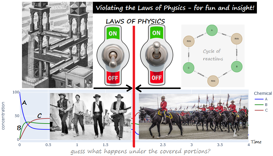
# ## Violating the Laws of Physics for Fun and Insight!
# ###  A cascade of reactions `A <-> B <-> C` , mostly in the forward direction
# ### [PART 1](#impossible_1_part1) : the above, together with a PHYSICALLY-IMPOSSIBLE "closing" of the cycle with :
# #### `C <-> A`,  *ALSO* mostly in the forward direction (never mind the laws of thermodymics)!
# ### [PART 2](#impossible_1_part2) : restoring the law of physics (by letting `C <-> A` adjust its kinetics based on the energy difference.)
# 
# All 1st-order kinetics.    
# 
# LAST REVISED: May 25, 2023

# ![Temporarily suspending the Laws of Physics](../../docs/impossible_1.png)

# In[1]:


import set_path      # Importing this module will add the project's home directory to sys.path


# In[2]:


from experiments.get_notebook_info import get_notebook_basename

from src.modules.reactions.reaction_data import ReactionData as chem
from src.modules.reactions.reaction_dynamics import ReactionDynamics
from src.modules.numerical.numerical import Numerical as num

import numpy as np
import plotly.express as px
import plotly.graph_objects as go
from src.modules.visualization.graphic_log import GraphicLog


# In[3]:


# Initialize the HTML logging
log_file = get_notebook_basename() + ".log.htm"    # Use the notebook base filename for the log file

# Set up the use of some specified graphic (Vue) components
GraphicLog.config(filename=log_file,
                  components=["vue_cytoscape_1"],
                  extra_js="https://cdnjs.cloudflare.com/ajax/libs/cytoscape/3.21.2/cytoscape.umd.js")


# ### Initialize the system

# In[4]:


# Initialize the system
chem_data = chem(names=["A", "B", "C"])

# Reaction A <-> B, mostly in forward direction (favored energetically)
# Note: all reactions in this experiment have 1st-order kinetics for all species
chem_data.add_reaction(reactants="A", products="B",
                       forward_rate=9., reverse_rate=3.)

# Reaction B <-> C, also favored energetically
chem_data.add_reaction(reactants="B", products="C",
                       forward_rate=8., reverse_rate=4.)


# # <a name="impossible_1_part1"></a> Part 1 - "Turning off the Laws of Physics"!

# In[5]:


# LET'S VIOLATE THE LAWS OF PHYSICS!
# Reaction C <-> A, also mostly in forward direction - MAGICALLY GOING "UPSTREAM" from C, to the higher-energy level of "A"
chem_data.add_reaction(reactants="C" , products="A",
                       forward_rate=3., reverse_rate=2.) # PHYSICALLY IMPOSSIBLE! Future versions of Life123 may flag this!

chem_data.describe_reactions()

# Send the plot of the reaction network to the HTML log file
graph_data = chem_data.prepare_graph_network()
GraphicLog.export_plot(graph_data, "vue_cytoscape_1")


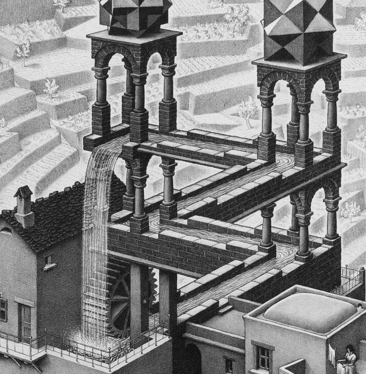
# # Notice the absurdity of the energy levels always going down, throughout the cycle (like in an Escher painting!)

# ![Energy levels always going down](../../docs/impossible_1b.jpg)

# ### Set the initial concentrations of all the chemicals

# In[6]:


initial_conc = {"A": 100., "B": 0., "C": 0.} 
initial_conc


# In[7]:


dynamics = ReactionDynamics(reaction_data=chem_data)
dynamics.set_conc(conc=initial_conc, snapshot=True)
dynamics.describe_state()


# In[8]:


dynamics.set_diagnostics()       # To save diagnostic information about the call to single_compartment_react()

# All of these settings are currently close to the default values... but subject to change; set for repeatability
dynamics.set_thresholds(norm="norm_A", low=0.5, high=0.8, abort=1.44)
dynamics.set_thresholds(norm="norm_B", low=0.08, high=0.5, abort=1.5)
dynamics.set_step_factors(upshift=1.1, downshift=0.4, abort=0.3)
dynamics.set_error_step_factor(0.2)

dynamics.single_compartment_react(initial_step=0.001, target_end_time=2.0,
                                  variable_steps=True, explain_variable_steps=False)


# In[9]:


dynamics.plot_curves()


# In[10]:


# dynamics.explain_time_advance()

# dynamics.get_history()


# ### It might look like an equilibrium has been reached.  But NOT!  Verify the LACK of final equilibrium state:

# In[11]:


dynamics.is_in_equilibrium()


# ## Not surprisingly, none of the reactions of this physically-impossible hypothetical system are in equilibrium
# ### Even though the concentrations don't change, it's NOT from equilibrium in the reactions - but rather from a balancing out of consuming and replenishing across reactions. 
# #### Consider, for example, the concentrations of `A` at the end time, and contributions to its change ("Delta A") from _individual_ reactions affecting `A`, as available from the diagnostic data:

# In[12]:


dynamics.get_diagnostic_rxn_data(rxn_index=0, tail=1)


# In[13]:


dynamics.get_diagnostic_rxn_data(rxn_index=2, tail=1)


# ### Looking at the last row from each of the 2 dataframes above, one case see that, at every reaction cycle, [A] gets reduced by 0.914286 by the reaction `A <-> B`, while simultaneously getting increased by the SAME amount by the (fictional) reaction `C <-> A`.   
# ### Hence, the concentration of A remains constant - but none of the reactions is in equilibrium!

# In[ ]:





# # <a name="impossible_1_part2"></a> PART 2 - Let's restore the Laws of Physics!

# In[14]:


chem_data.describe_reactions()


# In[15]:


dynamics.clear_reactions()       # Let's start over with the reactions  (without affecting the data from the reactions)


# In[16]:


# For the reactions A <-> B, and B <-> C, everything is being restored to the way it was before
chem_data.add_reaction(reactants="A", products="B",
                       forward_rate=9., reverse_rate=3.)

# Reaction , also favored energetically
chem_data.add_reaction(reactants="B", products="C",
                       forward_rate=8., reverse_rate=4.)


# In[17]:


chem_data.describe_reactions()


# In[18]:


# But for the reaction C <-> A, this time we'll "bend the knee" to the laws of thermodynamics!
# We'll use the same forward rate as before, but we'll let the reverse rate be picked by the system, 
# based of thermodynamic data consistent with the previous 2 reactions : i.e. an energy difference of -(-2,723.41 - 1,718.28) = +4,441.69 (reflecting the  
# "going uphill energetically" from C to A
chem_data.add_reaction(reactants="C" , products="A",
                       forward_rate=3., Delta_G=4441.69)   # Notice the positive Delta G: we're going from "C", to the higher-energy level of "A"


# In[19]:


chem_data.describe_reactions()


# # Notice how, now that we're again following the laws of thermodynamics, the last reaction is mostly IN REVERSE (low K < 1), as it ought to be! 
# #### (considering how energetically unfavorable it is)

# ### Now, let's continue with this "legit" set of reactions, from where we left off in our fantasy world at time t=2:

# In[20]:


dynamics.single_compartment_react(initial_step=0.01, target_end_time=4.0,
                                  variable_steps=True, explain_variable_steps=False)

#dynamics.explain_time_advance()

#dynamics.get_history()


# In[21]:


fig0 = dynamics.plot_curves(suppress=True)   # Prepare, but don't show, the main plot


# In[22]:


# Add a second plot, with a vertical gray line at t=2
fig1 = px.line(x=[2,2], y=[0,100], color_discrete_sequence = ['gray'])

# Combine the plots, and display them
all_fig = go.Figure(data=fig0.data + fig1.data, layout = fig0.layout)    # Note that the + is concatenating lists
all_fig.update_layout(title="On the left of vertical gray line: FICTIONAL world; on the right: REAL world!")
all_fig.show()


# ### Notice how [A] drops at time t=2, when we re-enact the Laws of Physics, because A no longer receives the extra boost from the previous mostly-forward (and thus physically-impossible given the unfavorable energy levels!) reaction `C <-> A`.   
# ### Back to the real world, that (energetically unfavored) reaction now mostly goes IN REVERSE; hence, the boost in [C] as well

# ### Now, we have a REAL equilibrium!

# In[23]:


dynamics.is_in_equilibrium()


# ### The fact that individual reactions are now in actual, real equilibrium, can be easily seen from the last rows in the diagnostic data.  Notice all the delta-concentration values at the final times are virtually zero:

# In[24]:


dynamics.get_diagnostic_rxn_data(rxn_index=0, tail=1)


# In[25]:


dynamics.get_diagnostic_rxn_data(rxn_index=1, tail=1)


# In[26]:


dynamics.get_diagnostic_rxn_data(rxn_index=2, tail=1)


# In[ ]: